The first time I ran an Apache Spark job, it was 2015. We had a batch ETL pipeline on Hadoop MapReduce that took 14 hours to process a day’s worth of clickstream data. Our data engineering lead had been pushing to migrate to Spark for months. I was skeptical because I had a healthy distrust of “10x faster” claims from any technology vendor.
The first Spark run finished in 47 minutes. That was not a benchmark. That was the same job, the same data, same cluster. We shipped the migration in three weeks.
Spark remains the dominant engine for large-scale data processing more than a decade after its Berkeley origins, and understanding its architecture is foundational knowledge for anyone doing serious data engineering. Here is how it actually works.
Why Spark Beat Hadoop MapReduce
Before going into Spark’s architecture, it is worth understanding why Spark replaced Hadoop MapReduce for most workloads.
MapReduce processes data in two phases: Map and Reduce. Every intermediate result gets written to HDFS disk between stages. If you have a pipeline with 10 stages, you read and write disk 10 times. For iterative algorithms (machine learning, graph computation), this is brutal. A k-means clustering algorithm that needs 100 iterations reads and writes HDFS 200 times.
Spark’s key innovation was in-memory processing. Instead of materializing every intermediate result to disk, Spark keeps data in memory as much as possible across multiple operations. For iterative algorithms, this is the difference between hours and minutes. For single-pass ETL, the speedup is smaller but still significant because you eliminate most of the HDFS I/O overhead.
The second key innovation was the unified programming model. MapReduce does map and reduce. That is it. Anything more complex requires chaining multiple MapReduce jobs. Spark gives you a rich functional API (map, filter, join, groupBy, window functions, SQL, ML, graph algorithms) in a single framework, with a single execution model underneath.
The Core Architecture: Driver, Executors, and Cluster Manager
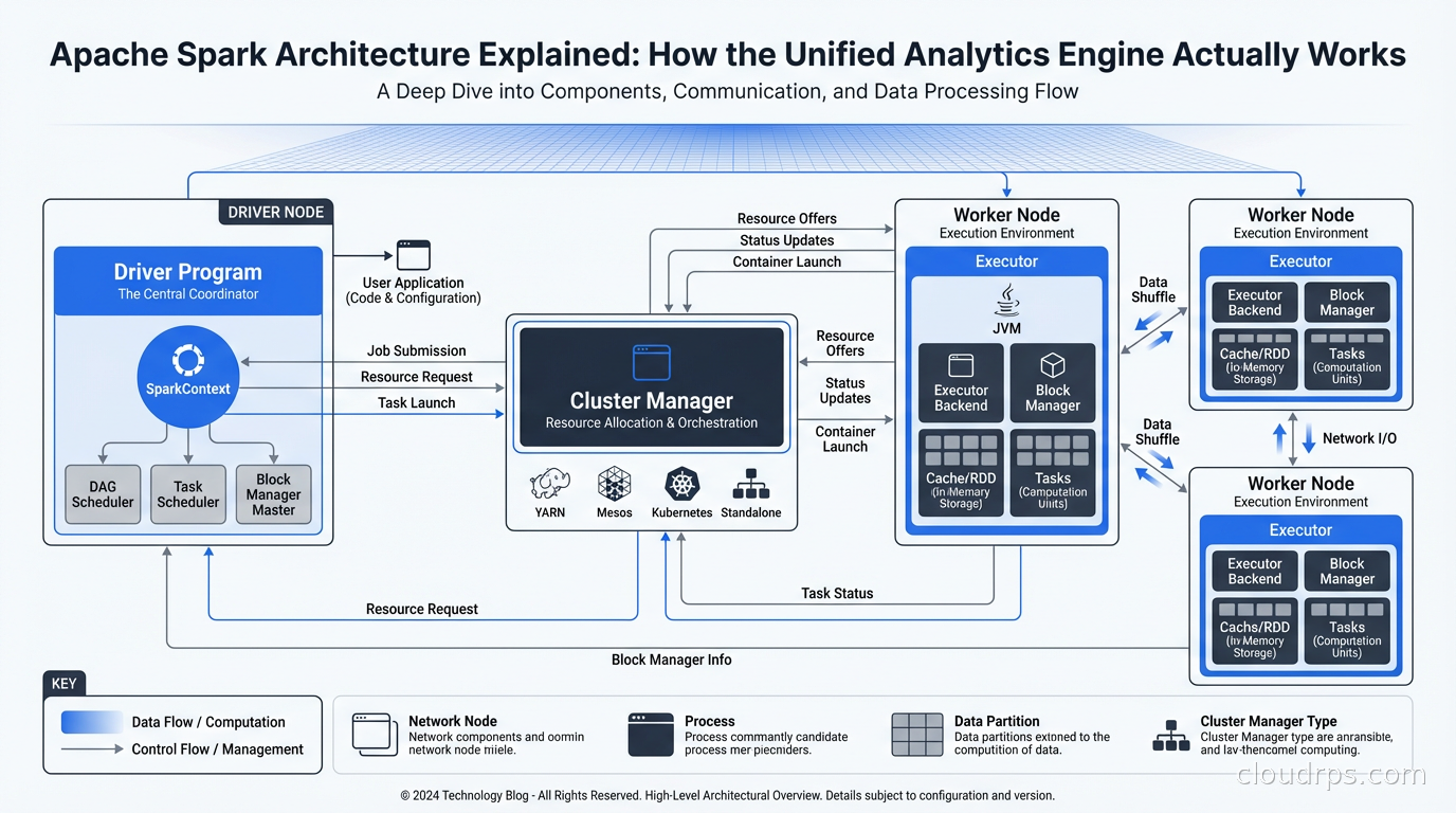
Every Spark application runs with the same three-layer architecture.
The Driver Program: This is your application. Whether you are running a PySpark script, a Spark SQL query, or a Spark Streaming job, there is one driver process that owns the application lifecycle. The driver runs your main() function, creates the SparkContext (or SparkSession in modern Spark), and coordinates all execution. The driver is responsible for planning the execution DAG, scheduling tasks on executors, and collecting results.
The Cluster Manager: Spark is decoupled from any specific cluster manager. It supports standalone mode (Spark’s own scheduler), YARN (Hadoop’s resource manager), Mesos (largely deprecated), and Kubernetes. The cluster manager’s job is to allocate resources (CPU and memory) for Spark executors. Spark requests resources from the cluster manager at application startup, runs its work, and releases them when done.
Executors: These are the processes that actually do the work. Each executor runs on a worker node, holds a slice of your data in memory (or on disk when memory spills), and executes the tasks the driver sends it. Executors are the unit of parallelism. A Spark job with 100 executor cores can run 100 tasks simultaneously.
The driver coordinates, the executors compute. This separation is clean. It also means the driver is a single point of failure for the application, which is worth knowing when you are thinking about fault tolerance.
RDDs, DataFrames, and Datasets: The Data Abstractions
Spark has three data abstractions, and understanding their history explains why the modern API looks the way it does.
RDDs (Resilient Distributed Datasets): The original Spark abstraction. An RDD is an immutable, distributed collection of objects. “Resilient” means Spark can recompute lost partitions by retracing the lineage of transformations that produced them. RDDs are the foundation of everything Spark does, but working with them directly is verbose and the optimizer cannot do much to help you.
DataFrames: Introduced in Spark 1.3. A DataFrame is an RDD of rows with a known schema. This is the “bring your own schema” moment that changed everything. Because Spark knows the schema, the Catalyst Optimizer can make intelligent decisions about execution order, predicate pushdown, column pruning, and join strategies. DataFrames also enabled SQL queries via SparkSQL. The API looks like Pandas but runs distributed across a cluster.
Datasets: Strongly typed DataFrames, available in Scala and Java (not Python, where DataFrames are already the idiomatic API). Datasets give you compile-time type safety while still going through the Catalyst Optimizer. In practice, most Python data engineers work with DataFrames and never touch the Dataset API.
My recommendation: use the DataFrame/SQL API unless you have a specific reason to drop down to RDDs. The optimizer improvements alone make DataFrames significantly faster for most workloads.
Lazy Evaluation and the DAG
This is the conceptual key to understanding how Spark executes.
When you write a Spark transformation (filter, map, join, groupBy), Spark does not execute it immediately. It builds a logical plan. When you finally call an action (count, collect, write), Spark takes the entire accumulated plan, optimizes it, and executes it all at once.
This approach is called lazy evaluation, and it enables powerful optimizations. Consider this:
df = spark.read.parquet("s3://bucket/data/")
    .filter(col("region") == "us-east-1")
    .select("user_id", "event_type", "timestamp")
    .groupBy("user_id")
    .agg(count("event_type").alias("event_count"))
When Spark optimizes this plan, it can push the filter and column selection down to the Parquet reader. Instead of reading all columns from all rows and then filtering, it reads only the three needed columns and skips any row groups that cannot contain region == "us-east-1". For a large dataset, this might reduce the data read from S3 by 90 percent.
This optimization is the Catalyst Optimizer’s job. It transforms your logical plan through several phases: analysis, logical optimization, physical planning, and code generation. The physical plan is what actually runs. Tungsten (Spark’s low-level execution engine) takes the physical plan and generates JVM bytecode optimized for the data types in your schema.
The execution of a Spark job is represented as a Directed Acyclic Graph (DAG) of stages. A stage is a set of transformations that can run without a shuffle. Whenever Spark needs to redistribute data across the cluster (a join, a groupBy, a repartition), it creates a stage boundary and performs a shuffle.
Shuffles are expensive. They involve serializing data, writing it to disk, transferring it across the network, and reading it on the destination side. Minimizing unnecessary shuffles is one of the most impactful Spark performance optimizations.
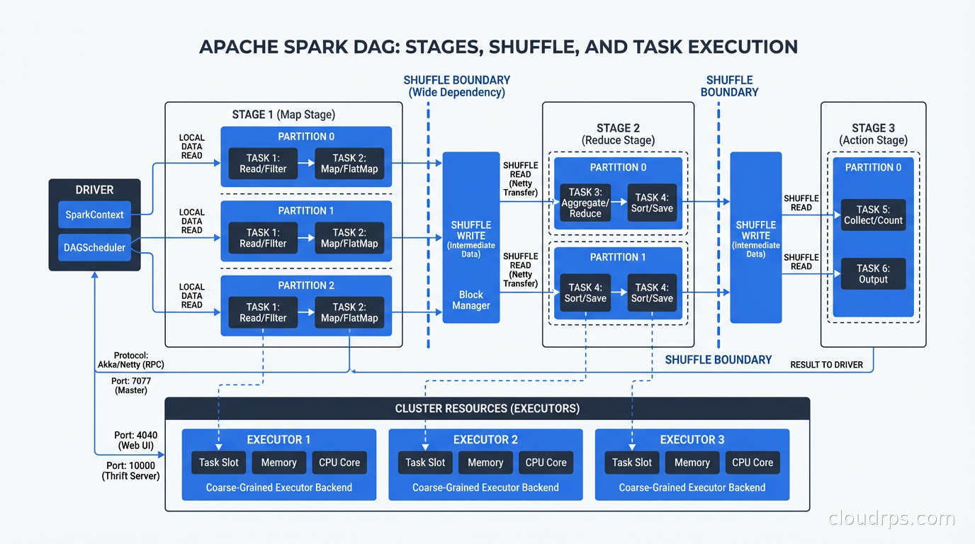
Partitioning: The Foundation of Parallelism
Every Spark DataFrame is divided into partitions. A partition is a chunk of data that lives on one executor and is processed by one task. If you have 200 partitions and 100 executor cores, Spark runs 100 tasks in the first wave and 100 in the second wave.
Getting partitioning right is one of the most important tuning levers you have.
Too few partitions: If you have 10 partitions and 100 executor cores, 90 cores sit idle. You are leaving parallelism on the table. This often happens when you read a small number of large files.
Too many partitions: If you have 100,000 partitions and 100 executor cores, you spend most of your time on task scheduling overhead rather than actual computation. Partitions smaller than 128MB are usually too small.
After a shuffle (join, groupBy), Spark uses spark.sql.shuffle.partitions to determine the output partition count. The default is 200. For small datasets this is way too many (creating thousands of tiny files). For large datasets it might be too few. Adaptive Query Execution (AQE), introduced in Spark 3.0, automatically coalesces shuffle partitions based on actual data size, which handles this reasonably well.
Data skew is the pathological partitioning case. A single partition has 10x the data of others because you have a hot key (think country = "US" in a groupBy on global data). That one task takes 10x longer than all others, and your job completion time is bottlenecked by the slow task. Solutions include salting the key, using skew hints (AQE handles some skew automatically), or repartitioning before the skew-inducing operation.
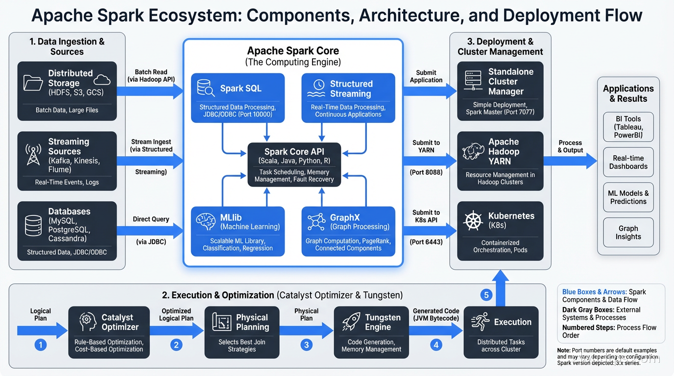
Spark SQL and the Warehouse Use Case
Spark SQL transformed Spark from an ETL tool into a general-purpose analytics engine. You can query any DataFrame with standard SQL:
spark.sql("""
    SELECT user_id, sum(revenue) as total_revenue
    FROM events
    WHERE event_date >= '2025-01-01'
    GROUP BY user_id
    HAVING sum(revenue) > 1000
""")
This goes through the same Catalyst Optimizer path as the DataFrame API. You can mix SQL and DataFrame operations freely.
For organizations running a data lakehouse architecture, Spark is the dominant query engine for transformation workloads. Apache Iceberg tables can be read and written directly from Spark with full ACID semantics. Spark handles the heavy transformation and aggregation work, while Iceberg provides the table format that makes concurrent reads and writes safe.
Spark is also the primary engine for data lake transformation at scale. If you are reading raw files from S3, transforming them, and writing clean tables, Spark is the standard choice for anything above moderate scale.
Structured Streaming: Real-Time with a Batch API
Spark Structured Streaming treats a real-time stream as an unbounded DataFrame. You write the same transformations you would write for batch data, and Spark handles the incremental execution continuously.
The programming model is genuinely elegant. A streaming query looks almost identical to a batch query:
stream_df = spark.readStream.format("kafka").option("subscribe", "events").load()

result = stream_df.groupBy(window("timestamp", "5 minutes"), "user_id").count()

result.writeStream.outputMode("update").format("delta").start()
Spark manages checkpointing (tracking what data has been processed), exactly-once semantics via transactional sinks, and watermarking (handling late-arriving data).
For stream processing architectures that need both batch and streaming in one framework, Spark Structured Streaming is the practical choice. It is not as low-latency as Apache Flink (Flink can operate at sub-second latency, while Spark’s micro-batch model typically means 100ms to 1s latency), but for workloads where seconds-level latency is acceptable, Spark avoids the operational complexity of running two separate systems.
Deployment: Where Spark Runs
Databricks: The dominant managed Spark platform. Databricks was founded by Spark’s original creators and contributes heavily to the open-source project. Their platform adds a collaborative notebook environment, managed clusters with autoscaling, Delta Lake (their open-source table format), Unity Catalog for governance, and Photon (a vectorized execution engine written in C++ that accelerates SQL workloads). Most large enterprises doing Spark at scale are on Databricks. The cost premium over self-managed Spark on YARN or Kubernetes is real but the operational savings usually justify it.
Amazon EMR: AWS’s managed Hadoop/Spark platform. You get managed Spark clusters on EC2 with tight integration to S3, Glue, Athena, and the rest of the AWS ecosystem. EMR Serverless removes cluster management entirely for batch workloads. Good choice if you are AWS-first and want to avoid the Databricks licensing conversation.
Google Dataproc: GCP’s managed Spark service. Similar to EMR. Tight integration with BigQuery and GCS. Dataproc Serverless for Spark is competitive with EMR Serverless.
Spark on Kubernetes: Increasingly common for organizations that already operate Kubernetes clusters and want to avoid separate cluster managers. Spark jobs run as Kubernetes pods, using standard K8s resource management. Works well, but requires more configuration than managed services. The Kubernetes ecosystem handles scheduling, monitoring, and autoscaling.
Self-managed YARN: Still common in organizations with existing Hadoop clusters. If you have HDFS and YARN already, running Spark on top is straightforward. But greenfield deployments rarely start here anymore.
Performance Tuning: The Levers That Actually Matter
There are dozens of Spark configuration parameters. Here are the ones that actually move the needle.
Memory allocation: Each executor has a heap divided into execution memory (for shuffles and aggregations) and storage memory (for cached data). The split is managed by spark.memory.fraction and spark.memory.storageFraction. The defaults are reasonable. Only tune these if you are seeing excessive GC pauses or OOM errors.
Parallelism: Set spark.default.parallelism to 2-3x your total executor cores. For SQL workloads, set spark.sql.shuffle.partitions to match your data volume (roughly 100MB to 200MB per partition after the shuffle). Enable AQE (spark.sql.adaptive.enabled=true, which is default since Spark 3.2) to let Spark tune shuffle partitions automatically.
Caching: Use df.cache() when you reuse a DataFrame multiple times. Do not cache everything. Cache only DataFrames that are expensive to compute and reused at least twice. Spark’s memory is finite and evicting the wrong cached DataFrame causes recomputation that is slower than not caching.
File formats: Always use Parquet or ORC for storage, not CSV or JSON. Parquet’s columnar format enables predicate pushdown and column pruning that can reduce I/O by orders of magnitude. If you are writing output files, control the number of output files with repartition() or coalesce() before writing to avoid the “small files problem”.
Broadcast joins: If one side of a join is small (under spark.sql.autoBroadcastJoinThreshold, default 10MB), Spark will automatically broadcast it to all executors and avoid the shuffle entirely. For joins with lookup tables or dimension tables, this is a huge win.
MLlib and Machine Learning at Scale
Spark MLlib is the machine learning component of the Spark ecosystem. It provides distributed implementations of common ML algorithms: linear regression, logistic regression, decision trees, random forests, k-means clustering, and more.
MLlib’s Pipelines API (transformers, estimators, pipeline stages) influenced the design of scikit-learn’s Pipeline interface. It is the right tool when your training data does not fit in memory on a single machine or when you need to apply ML transformations within a Spark data pipeline.
For deep learning and GPU workloads, MLlib is not the answer. You would train on GPU clusters (using PyTorch or TensorFlow) and use Spark for feature engineering and data preprocessing. The MLOps pipeline connects the two: Spark for feature computation, a training framework for model training, and then Spark again for batch inference at scale. If you are managing production ML pipelines, the MLOps practices and infrastructure around feature stores and model serving are where Spark fits in.
For integrating real-time data changes into Spark pipelines, Change Data Capture with Debezium is the standard approach. CDC streams database changes into Kafka, and Spark Structured Streaming consumes those events to maintain materialized views or trigger downstream processing.
When to Use Spark vs. Alternatives
Spark is not always the right tool. Here is my honest take on when to use it and when not to.
Use Spark when: You have truly large datasets (hundreds of GB to TB+), you need unified batch and streaming in one system, you need the ML integration, or you are already on a Databricks or EMR platform where Spark is the default.
Use Flink instead when: You need sub-second streaming latency, you have complex stateful streaming logic, or you need exactly-once semantics in streaming without micro-batch constraints.
Use DuckDB instead when: Your dataset fits comfortably in memory (or can be processed file by file). DuckDB running on a single large machine is faster than Spark for datasets under ~100GB, costs less, and requires zero cluster management. The rise of DuckDB has genuinely shifted where the Spark boundary makes sense downward.
Use Trino/Presto instead when: You need interactive, low-latency SQL queries against large datasets and do not need transformation workloads. Trino is optimized for query latency. Spark is optimized for throughput.
Use BigQuery or Snowflake instead when: You are primarily doing SQL analytics and want a fully managed warehouse without any infrastructure or tuning work. Managed warehouses have closed the performance gap with self-managed Spark for pure SQL workloads.
The practical answer for most data engineering teams: Spark (usually via Databricks or EMR) for complex ETL and transformation at scale, plus a purpose-built tool for interactive queries or specialized streaming requirements.
A War Story: Migrating 3 TB of Daily ETL
At a retail company a few years back, we inherited a custom batch processing system written in Java that read from MySQL, applied transformations, and wrote results to a PostgreSQL data warehouse. It ran nightly, took 6 hours, and failed about once per week with cryptic out-of-memory errors.
The underlying data volume was 3TB of raw transaction data daily. The transformations included sessionization (grouping events by user session), attribution (which marketing touchpoint drove a conversion), and daily aggregation at multiple levels.
We migrated to Spark on EMR over about three months. The first month was building the Spark jobs and getting them working correctly (testing ETL logic is underrated as a skill). The second month was tuning: the sessionization logic had terrible data skew because power users generated 100x the events of average users. We solved it with a two-phase approach: compute partial session statistics in parallel per user partition, then merge.
The final result: 6 hours became 45 minutes. Weekly failures became zero in 4 months of production operation. The team maintaining it went from five engineers who understood the Java codebase to any data engineer comfortable with PySpark. That maintainability benefit often gets undersold in migration business cases, but it is real.
Get Cloud Architecture Insights
Practical deep dives on infrastructure, security, and scaling. No spam, no fluff.
By subscribing, you agree to receive emails. Unsubscribe anytime.