Big Data, Hadoop, and MapReduce: The Complete Architecture Guide

I still remember the first time someone told me we needed to process 40 terabytes of clickstream data overnight. It was 2009, I was running architecture for a retail analytics platform, and our Oracle RAC cluster was wheezing under the load like a chain smoker climbing stairs. A colleague dropped the word “Hadoop” in a meeting, and within six months our entire data processing pipeline looked completely different.

Hadoop changed the industry. Not because it was elegant (it was anything but), and not because it was fast in any conventional sense. It changed things because it made a radical bet: instead of moving data to the compute, move the compute to the data. That bet paid off spectacularly for an entire generation of data infrastructure.

This guide is what I wish someone had handed me back in 2009. We’ll walk through the actual architecture, the pieces that matter, the pieces that don’t anymore, and where all of this fits in a world that’s moved well beyond batch processing.

The Problem Hadoop Was Built to Solve

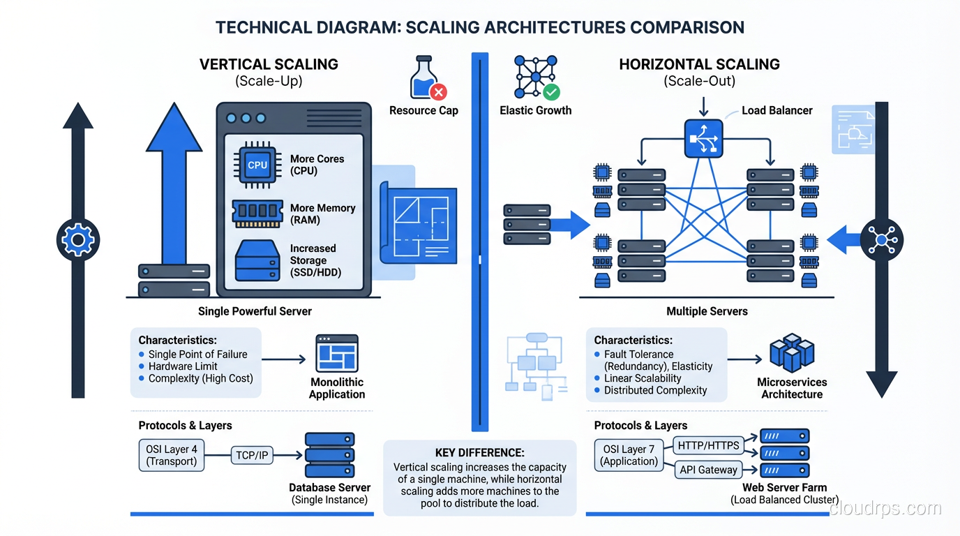
Before Hadoop, scaling data processing meant buying bigger machines. You hit a wall on a single server, so you bought one with more RAM, more CPUs, faster disks. This is vertical scaling, and it has a hard ceiling, both technically and financially. I’ve signed purchase orders for single database servers that cost more than most people’s houses.

The alternative was horizontal scaling, spreading work across many commodity machines. But distributed computing is hard. Really hard. You have to deal with network partitions, node failures, data locality, coordination overhead, and a dozen other problems that don’t exist when everything runs on one box.

Hadoop’s genius was abstracting all of that away behind two clean primitives: a distributed filesystem (HDFS) and a parallel processing framework (MapReduce). You write your logic as map and reduce functions, and the framework handles the rest: splitting the data, shipping your code to the right nodes, handling retries when machines die, merging results.

HDFS: The Foundation Layer

The Hadoop Distributed File System is where everything starts. HDFS takes large files, chops them into blocks (128MB by default, though I’ve run clusters with 256MB and even 512MB blocks for specific workloads), and distributes those blocks across a cluster of commodity machines.

NameNode and DataNodes

HDFS runs on a master-worker architecture. The NameNode is the master; it keeps track of which blocks live on which DataNodes, manages the filesystem namespace, and handles client requests. DataNodes are the workers. They store the actual data blocks and serve read/write requests.

Here’s the thing nobody tells you in the documentation: the NameNode is a single point of failure, and it keeps its entire metadata structure in RAM. I learned this the hard way when a NameNode ran out of heap space on a cluster with 200 million small files. The entire cluster went down. This is why HDFS works best with large files, since fewer files means less metadata, which means less pressure on the NameNode.

The HA (High Availability) NameNode setup with a standby node and shared edit logs via JournalNodes was a game-changer when it landed. Before that, we were running with our fingers crossed and very aggressive backup scripts.

Replication and Data Locality

By default, HDFS replicates every block three times across different nodes. The placement policy is smarter than it looks: the first replica goes on the local node, the second on a different rack, and the third on another node in that second rack. This gives you both node-level and rack-level fault tolerance.

But replication isn’t just about reliability. It’s about data locality, which is the entire reason Hadoop performs. When MapReduce schedules a task, it tries to run the task on a node that already has the data block locally. If that node is busy, it tries another node on the same rack. Network I/O across racks is the slowest part of the pipeline, so keeping computation local to the data is where the real performance gains come from.

I’ve seen well-tuned clusters achieve over 90% data locality on their map tasks. Poorly configured clusters (wrong block sizes, unbalanced DataNodes, too few replicas) might hit 40%. That difference translates directly into job completion time.

MapReduce: The Processing Engine

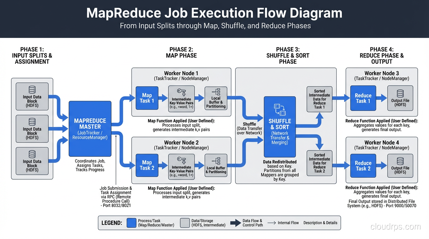
MapReduce is a programming model that breaks computation into two phases: map and reduce. The map phase processes input data in parallel across the cluster, producing intermediate key-value pairs. The reduce phase aggregates those intermediate results by key to produce the final output.

How a MapReduce Job Actually Executes

Let me walk through what actually happens when you submit a MapReduce job, because the documentation glosses over the details that matter operationally.

1. Input splitting: The framework examines your input data and creates one input split per HDFS block (roughly). Each split becomes one map task.

2. Map phase: Each map task reads its split, applies your map function to every record, and writes intermediate key-value pairs to local disk, not to HDFS. This is important. Intermediate data is local, temporary, and not replicated.

3. Shuffle and sort: This is the phase nobody talks about, and it’s where most MapReduce jobs actually spend their time. The framework partitions the intermediate data by key, sorts it, and transfers it across the network to the correct reduce tasks. I’ve debugged more performance problems in the shuffle phase than in map and reduce combined.

4. Reduce phase: Each reducer receives all values for a given set of keys, applies your reduce function, and writes the output to HDFS.

The Shuffle Is Where Jobs Go to Die

I cannot overstate how critical the shuffle phase is. The shuffle involves disk I/O on the map side (spilling sorted runs to disk), network I/O (transferring data to reducers), and disk I/O plus merge operations on the reduce side.

Common problems I’ve diagnosed in the shuffle phase:

• Too many reducers causing excessive network connections and small output files
• Too few reducers causing memory pressure and long reduce times
• Skewed keys where one reducer gets 80% of the data while the others sit idle
• Insufficient sort buffer causing excessive disk spills on the map side

The io.sort.mb and io.sort.factor settings are among the most impactful tuning knobs in the entire Hadoop ecosystem. I’ve seen jobs go from 4 hours to 45 minutes just by getting the shuffle configuration right.

YARN: The Resource Manager

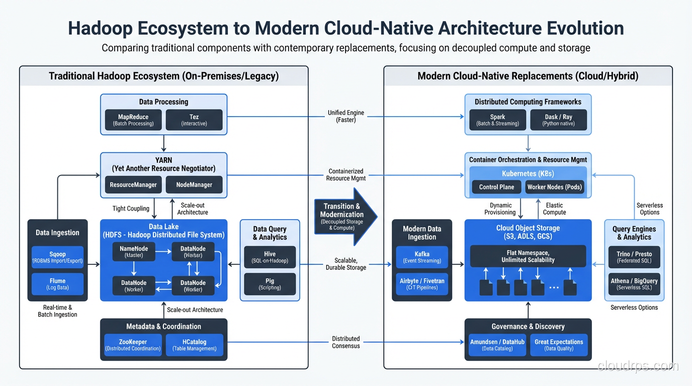
In Hadoop 1.x, MapReduce was both the processing engine and the resource manager. This was a terrible design, because it meant only MapReduce jobs could run on the cluster. YARN (Yet Another Resource Negotiator) decoupled resource management from processing, which opened the door for Spark, Tez, Flink, and every other processing framework that runs on Hadoop today.

YARN has a ResourceManager (cluster-wide) and NodeManagers (per-node). Applications request containers (bundles of CPU and memory) from the ResourceManager, and NodeManagers launch and monitor those containers.

The critical insight with YARN is that it turned Hadoop from a batch processing system into a general-purpose distributed computing platform. This is why Hadoop clusters survived long after MapReduce fell out of favor. The storage (HDFS) and resource management (YARN) layers still provided value, even after everyone switched to Spark for processing.

The Hadoop Ecosystem: What Matters and What Doesn’t

Over the years, the Hadoop ecosystem exploded into dozens of projects. Here’s my honest assessment of what still matters.

Still Relevant

• HDFS: Still the backbone of many data lake architectures. If you’re dealing with on-premises big data, HDFS is likely part of your stack. For more on how this fits into broader storage patterns, see data lake architecture.
• YARN: Still manages resources on Hadoop clusters, particularly for Spark workloads.
• Hive: SQL on Hadoop. The metastore component specifically has become a de facto standard for table metadata, even outside Hadoop.
• HBase: Column-family NoSQL database on HDFS. Still used for specific workloads needing random read/write access to large datasets.

Largely Replaced

• MapReduce as a processing engine: Spark does everything MapReduce does, faster, with a better programming model. I haven’t written a raw MapReduce job in production since 2016.
• Pig: The scripting layer for MapReduce. Dead.
• Oozie: Workflow scheduler. Replaced by Airflow, Dagster, and similar tools.
• Sqoop: Data import/export tool. Various better alternatives exist now.

The Concepts That Survived

Even if you never touch Hadoop directly, the architectural patterns it established are everywhere in modern data engineering:

• Data locality: Still the core principle behind systems like Spark, Presto, and Trino.
• Horizontal scaling on commodity hardware: This is now the default assumption for every distributed system.
• Schema-on-read: Hadoop normalized the idea of storing raw data and applying structure at query time. This directly led to the data lake pattern.
• Fault tolerance through replication and retry: Every modern distributed system uses some variant of this.

When Hadoop Still Makes Sense in 2026

I get asked this question constantly: “Should we still use Hadoop?” The honest answer is nuanced.

Hadoop makes sense when:

• You have massive on-premises data processing requirements and can’t (or won’t) move to the cloud
• You have existing investments in HDFS and Hive that are working well
• You need a shared storage layer for multiple processing engines (Spark, Presto, etc.)
• Regulatory requirements keep you on-premises with petabyte-scale data

Hadoop doesn’t make sense when:

• You’re starting from scratch. Use cloud-native services instead.
• Your data volumes are under a few terabytes. A single well-provisioned server handles that fine.
• You need real-time processing. Look at stream processing architectures instead.
• You don’t have the operational expertise to run a Hadoop cluster (and trust me, it takes a lot)

Architecture Patterns for Modern Big Data

If I were designing a big data architecture today, it wouldn’t look like a Hadoop cluster from 2012. But it would use many of the same principles.

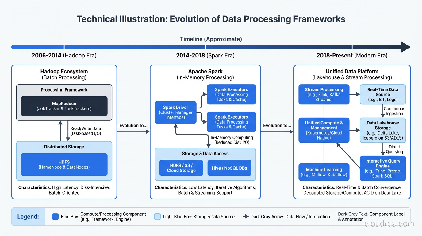
The Lakehouse Pattern

The modern evolution is the lakehouse, which combines the flexibility of a data lake with the performance and governance features of a data warehouse. You store data in open formats (Parquet, ORC) on object storage (S3, GCS, ADLS), use table formats like Delta Lake or Apache Iceberg for ACID transactions and schema evolution, and query with engines like Spark, Trino, or Dremio.

This is essentially what Hadoop promised, executed better with modern tooling.

Batch Plus Streaming

Most real architectures need both batch and stream processing. The Lambda architecture (batch layer plus speed layer) was the original answer to this. The Kappa architecture (everything as a stream) was the counter-proposal. In practice, most shops I work with end up with a pragmatic hybrid: streaming for low-latency use cases, batch for heavy analytics, with a shared storage layer underneath.

For deep dives on the streaming side, see my piece on stream processing with Kafka and Flink.

Storage Format Matters More Than You Think

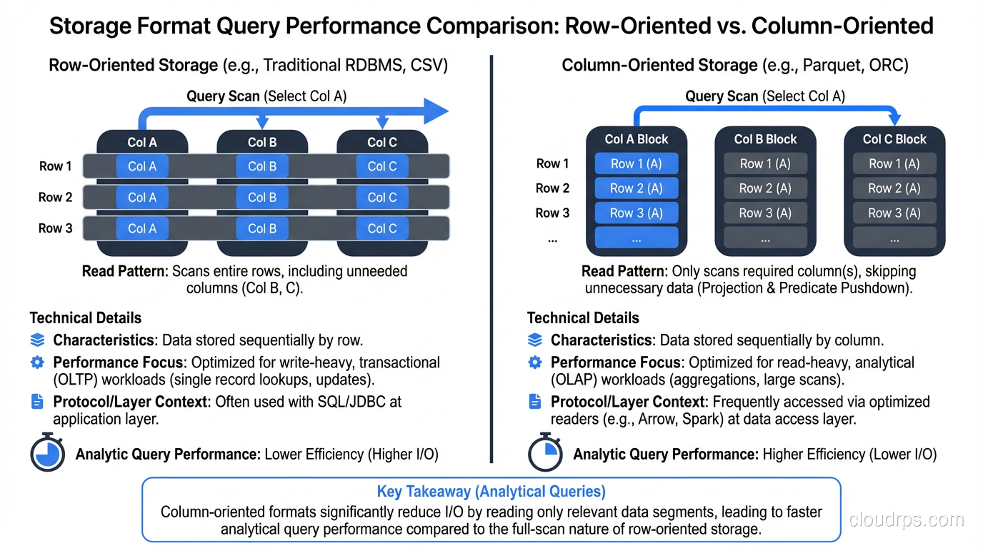
The choice between Parquet, ORC, Avro, and CSV has more impact on query performance than most people realize. Columnar formats like Parquet and ORC give you predicate pushdown, column pruning, and dramatically better compression ratios for analytical queries. I’ve seen query times drop by 10x just by converting CSV files to Parquet, with no other changes needed. For more on how storage formats interact with database design, check out columnar vs row databases.

Performance Tuning Lessons From the Trenches

After tuning hundreds of Hadoop jobs across dozens of clusters, here are the lessons that come up over and over.

Get Your Block Size Right

The default 128MB block size is fine for most workloads, but think about what it means. If you have millions of small files (say, 1KB each), each file becomes one block, each block becomes one map task, and you spend more time on task startup than actual processing. This is the “small files problem,” and it kills Hadoop performance. Solutions include using CombineFileInputFormat, merging files before ingestion, or using HBase for small-record workloads.

Memory Configuration Is Everything

The JVM heap settings for map and reduce tasks are the most commonly misconfigured parameters I see. Set them too low and you get OutOfMemoryErrors or excessive garbage collection. Set them too high and you waste cluster resources or starve other tasks.

My rule of thumb: map tasks get 1-2GB heap for most workloads. Reduce tasks get 2-4GB because they need to hold more data in memory during the merge phase. But always profile your actual jobs. These are starting points, not gospel.

Monitor the Right Metrics

The metrics that actually tell you something useful: data locality percentage, shuffle bytes (total and per-reducer), GC time as a percentage of task time, and speculative execution rate. If your speculative execution rate is high, you have stragglers, which usually means either data skew or hardware problems on specific nodes.

The Legacy and the Lesson

Hadoop taught an entire generation of engineers how to think about distributed data processing. The specific technology is fading (I’d estimate that new Hadoop deployments have dropped by 80% compared to five years ago), but the ideas are permanent fixtures in our field.

If you’re a younger engineer who never had to write a MapReduce job, count yourself lucky. But understand the model, because you’ll encounter its descendants everywhere: in Spark’s RDD lineage, in Flink’s parallel dataflows, in every cloud service that spreads your data across nodes and brings computation to it.

The machines got faster. The abstractions got better. But the fundamental challenge, processing more data than fits on one machine, hasn’t changed. Hadoop was one of the first practical answers to that challenge at scale, and its architectural DNA lives on in every big data system you’ll touch today.