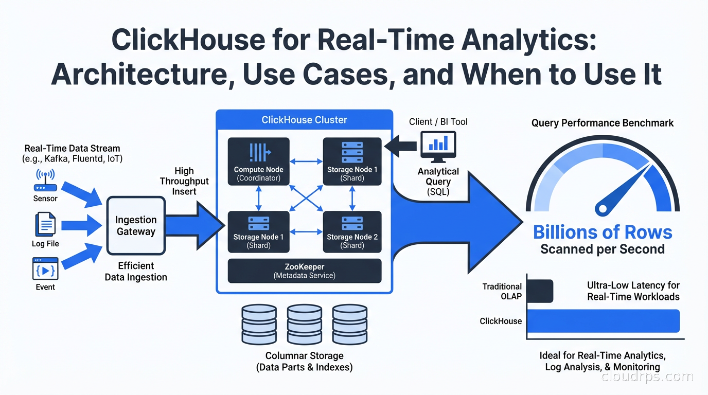
I used to think that if you needed sub-second analytics on billions of rows, you either spent a fortune on Snowflake, accepted Spark’s job startup latency, or engineered something custom and painful. Then I started using ClickHouse, and I discovered that it’s possible to run an aggregation query across 10 billion rows in under a second on a $200/month server. Not with caching, not with pre-aggregated materialized views (though those help), but with a direct scan of compressed columnar data.
ClickHouse is not new (Yandex open-sourced it in 2016), but it has reached a kind of inflection point in adoption. OpenAI uses it for observability. Netflix uses it for analytics. Cloudflare built their entire analytics product on it. Uber runs billions of rows through it daily. The tooling around ClickHouse has also matured: ClickHouse Cloud provides a fully managed offering, ClickPipes handles managed ingestion from Kafka and object storage, and the ecosystem of connectors and integrations has caught up with the major cloud data warehouses.
If you’re making decisions about your real-time analytics stack in 2026 and haven’t evaluated ClickHouse, you’re leaving performance and cost on the table.
The Architecture That Makes It Fast
ClickHouse is a column-oriented database, but “column-oriented” understates what makes it exceptional. Understanding the architecture explains the benchmark numbers.
In a row-oriented database like PostgreSQL, data is stored on disk row by row. When you query SELECT count(*), avg(revenue) FROM orders WHERE date > '2025-01-01', the database reads entire rows even though you only need two columns. For analytics on wide tables (50+ columns), you’re reading and decompressing data you don’t need.
In ClickHouse, each column is stored separately on disk. The same query reads only the date and revenue columns. On a table with 100 columns, that might mean reading 2% of the data a row-oriented database would read for the same query. For analytics workloads, this is a fundamental advantage.
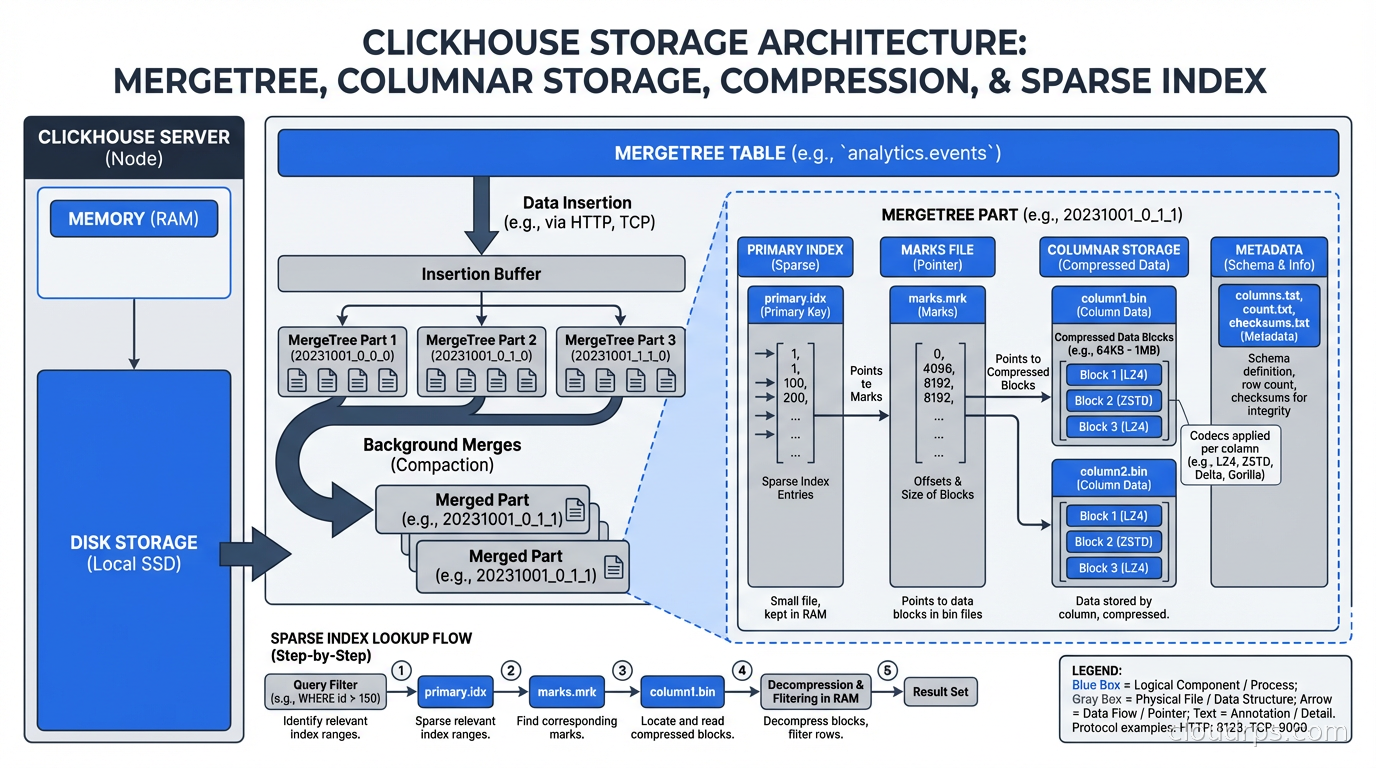
ClickHouse then applies aggressive compression column-by-column. Each column gets a codec chosen based on data type and distribution: LZ4 for general data, ZSTD for better compression ratios, Delta encoding for monotonically increasing time series (very effective for timestamps), DoubleDelta for second-order time series, Gorilla encoding for floating-point metrics. The default codecs achieve 5-10x compression on typical analytics data, which means more data fits in memory and in OS page cache. Less I/O means faster queries.
The MergeTree storage engine is the heart of ClickHouse. Data is written to parts (sorted by the primary key), and background merge operations periodically combine parts while maintaining sort order. This is similar to LSM trees but with different optimization targets: ClickHouse optimizes for scan performance at the cost of some write amplification and merge complexity.
Primary keys in ClickHouse work differently than in row-oriented databases. The primary key defines the sort order of data within parts and is used to skip blocks of data that can’t contain matching rows (sparse indexing). The primary key is NOT a uniqueness constraint. Choosing the right primary key for your query patterns is the single most important ClickHouse tuning decision.
Materialized Views and Continuous Aggregation
Where ClickHouse really pulls ahead for real-time analytics is its materialized view system, which works differently from the materialized views you know from PostgreSQL or Snowflake.
ClickHouse materialized views are triggers. When data is inserted into a source table, the materialized view definition runs against the new data and inserts the result into a target table. This happens synchronously at insert time. You get continuous, incremental aggregation with no separate processing job.
-- Source table: raw events
CREATE TABLE events (
    timestamp DateTime,
    user_id UInt64,
    event_type String,
    page String,
    session_id String
) ENGINE = MergeTree()
ORDER BY (timestamp, user_id);

-- Materialized view: pre-aggregate page views per minute
CREATE MATERIALIZED VIEW page_views_per_minute
ENGINE = SummingMergeTree()
ORDER BY (minute, page)
AS SELECT
    toStartOfMinute(timestamp) AS minute,
    page,
    count() AS views,
    uniqExact(user_id) AS unique_users
FROM events
GROUP BY minute, page;
Every event inserted into events automatically updates page_views_per_minute. Queries against the aggregated view scan a fraction of the data and return near-instantly. You get real-time dashboards backed by pre-aggregated data, updated as events arrive.
The AggregatingMergeTree and SummingMergeTree engines handle partial aggregates correctly during background merges, so your counts, sums, and cardinality estimates remain accurate even as the MergeTree engine merges parts in the background.
This pattern is how ClickHouse-based observability platforms work: raw events land in one table, dozens of materialized views aggregate them by different dimensions (by service, by error code, by time bucket, by user segment), and dashboards query the aggregated views for instant response.
ClickHouse vs. The Alternatives
The honest comparison against what you’re probably using:
vs. PostgreSQL: PostgreSQL is row-oriented and optimized for OLTP (lots of small writes and point queries). Running analytical queries on large PostgreSQL tables is painful: table scans are slow, PostgreSQL’s columnar extensions (timescaledb, cstore_fdw) help but add complexity, and the query planner makes different tradeoffs than an OLAP-focused engine. PostgreSQL is the right tool for your operational database; ClickHouse is the right tool for your analytics. They work well together via ClickHouse’s PostgreSQL integration for change data capture from Postgres into ClickHouse.
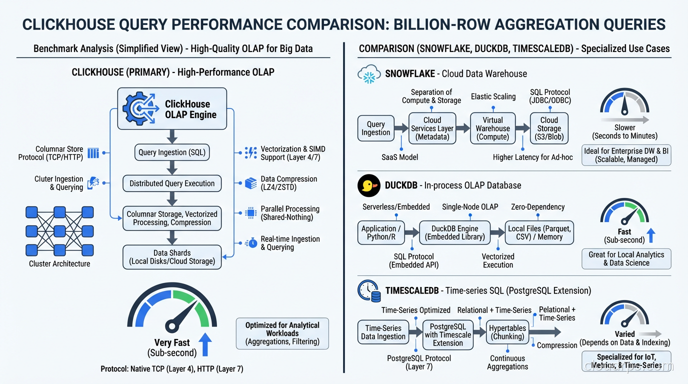
vs. DuckDB: DuckDB (which I covered in the embedded analytics guide) is excellent for single-node, in-process analytics. It’s better for local analysis, embedded in applications, or ad-hoc query workloads on files. ClickHouse is better for high-concurrency production analytics serving many users simultaneously, for ingesting data in real time, and for distributed scale. They’re complementary: use DuckDB for exploration and development, ClickHouse for production serving.
vs. Snowflake/BigQuery: These cloud data warehouses are excellent but expensive and optimized for batch ETL workloads rather than real-time ingestion. ClickHouse’s ingestion latency is seconds; Snowflake’s is minutes to hours for streaming loads. ClickHouse’s cost per query at scale is dramatically lower. The tradeoff: Snowflake and BigQuery have more mature governance features, better SQL compatibility, and more ecosystem integrations. For fresh real-time data at high query concurrency, ClickHouse wins decisively.
vs. TimescaleDB: TimescaleDB is PostgreSQL-based and excellent for time-series data with a strong time-series query model. ClickHouse scans time-series data faster than TimescaleDB at scale (benchmarks show 3-16x depending on the query). TimescaleDB has better SQL compatibility and is easier to integrate into PostgreSQL-centric toolchains. If you’re already on PostgreSQL and need better time-series performance, TimescaleDB is the lower-friction upgrade. If you’re starting fresh and need maximum performance, ClickHouse wins.
vs. Apache Druid: Druid is another high-performance OLAP database, popular for user-facing analytics products. ClickHouse is generally faster on scan-heavy analytics queries; Druid has more sophisticated data cube and rollup capabilities. ClickHouse is simpler to operate (Druid’s cluster has more moving parts: Broker, Coordinator, Historical, MiddleManager, Overlord). In 2026, ClickHouse has largely displaced Druid for new deployments.
Ingestion Patterns
ClickHouse handles ingestion differently than most databases, and understanding this prevents production surprises.
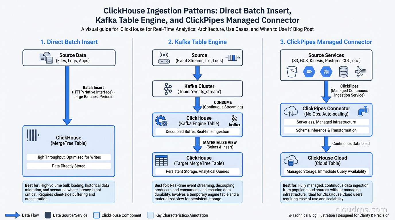
ClickHouse is optimized for batch inserts, not single-row inserts. Inserting one row at a time is an anti-pattern: each insert creates a new part, background merges work harder, and insert performance degrades. Target inserts of 1000-100,000 rows per batch, inserted every 100ms-10s.
For real-time ingestion from Kafka, ClickHouse has a native Kafka table engine:
CREATE TABLE kafka_events (
    timestamp DateTime,
    user_id UInt64,
    event_type String
) ENGINE = Kafka()
SETTINGS
    kafka_broker_list = 'kafka:9092',
    kafka_topic_list = 'events',
    kafka_group_name = 'clickhouse-consumer',
    kafka_format = 'JSONEachRow';
A materialized view then pushes from the Kafka table to your actual storage table. The Kafka table engine buffers messages and inserts them in batches, giving you the write pattern ClickHouse needs without forcing your producers to batch explicitly.
ClickPipes (ClickHouse Cloud’s managed ingestion) handles this infrastructure automatically, with source connectors for Kafka, Amazon Kinesis, Google Cloud Pub/Sub, and object storage formats. If you’re on ClickHouse Cloud, use ClickPipes rather than managing Kafka table engines yourself.
For CDC from operational databases, the pattern I described in the change data capture guide works perfectly with ClickHouse: Debezium publishes to Kafka, ClickHouse consumes from Kafka, and you have near-real-time analytics on data from your operational databases.
Operational Considerations
ClickHouse clusters have a few operational characteristics to plan around.
Replication uses ZooKeeper or ClickHouse Keeper. For production clusters with the ReplicatedMergeTree engine, you need a coordination service for metadata consistency. ClickHouse Keeper (ClickHouse’s own implementation of the ZooKeeper protocol) is the recommended choice now: it’s lighter weight and doesn’t require Java.
Sharding is manual. Unlike some distributed databases that handle sharding transparently, ClickHouse sharding is explicit. You create a Distributed table engine that routes queries across shards. Choosing the right sharding key is critical for query performance and avoiding hot shards. The sharding key should distribute data evenly and align with your query patterns (queries that filter on the sharding key can skip irrelevant shards).
Mutations are expensive. UPDATE and DELETE operations in ClickHouse are implemented as mutations: asynchronous operations that rewrite data parts. This is fundamentally different from OLTP databases. ClickHouse is not the right store for data that needs frequent updates to individual rows. If you need both OLAP analytics and mutable operational data, keep your mutable data in PostgreSQL and replicate it to ClickHouse for analytics.
Schema evolution is less flexible than cloud data warehouses. Adding columns is easy. Changing column types or dropping columns requires more care. ClickHouse’s ALTER operations are mostly metadata operations (fast) for adding columns, but data changes require rewrites.
Memory management matters. ClickHouse uses a lot of memory for query execution, particularly for aggregations over high-cardinality columns. The max_memory_usage setting per query and the max_server_memory_usage setting for the instance need tuning based on your hardware and query patterns. Queries that exceed memory limits fail; tune your memory or use approximate aggregation functions (like uniq instead of uniqExact for approximate cardinality).
Where ClickHouse Fits in Your Stack
The architectural pattern that I recommend for 2026: PostgreSQL (or another OLTP database) for operational data, Kafka for event streaming, ClickHouse for real-time analytics and observability. This is the stack used by companies serving billions of events per day.
ClickHouse is not a replacement for your operational database. It’s the analytics layer that lets your operational database focus on transactional workloads while ClickHouse handles the complex aggregations, funnel queries, cohort analyses, and time-series breakdowns that would crush your PostgreSQL instance.
The data observability use case is particularly compelling: ClickHouse handles the ingestion volume of observability data (logs, metrics, traces) that Elasticsearch and traditional databases struggle with at scale, and it does it cheaply. Many observability platforms have migrated their storage layer to ClickHouse in the last two years.
If you’re evaluating real-time analytics databases and haven’t run a ClickHouse benchmark against your actual data and queries, do it before making a decision. The performance numbers can be surprising in ways that change your architecture plans entirely.
Get Cloud Architecture Insights
Practical deep dives on infrastructure, security, and scaling. No spam, no fluff.
By subscribing, you agree to receive emails. Unsubscribe anytime.