Continuous Profiling in Production: Pyroscope, Parca, and Finding the CPU Hog You Never Knew You Had

Three years ago, I spent two weeks chasing a latency spike in a Go service that handled about 50,000 requests per minute. Metrics showed CPU at 60%. Distributed traces showed individual requests completing in 50-100ms. Nothing looked alarming. But p99 latency had quietly drifted from 200ms to 800ms over six months, and nobody could explain why.

Eventually, a junior engineer stumbled onto the answer by running pprof manually during a production traffic window. The culprit: a string formatting function inside a log statement, called on every request, constructing a detailed audit log that we were then immediately discarding because the log level was INFO and production was set to WARN. The garbage collector was thrashing. The fix was four lines. The discovery took two weeks.

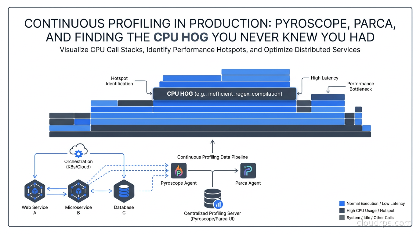
That is the problem continuous profiling solves. Metrics tell you something is wrong. Traces show you which request was slow. But profiles tell you exactly which line of code is consuming CPU, which object is filling your heap, which goroutine is stuck waiting. Without continuous profiling deployed before the incident, you are flying blind into production performance problems.

What Continuous Profiling Actually Is

Traditional profiling means someone runs a profiler against a service, collects data for 30 seconds, analyzes it, then stops. That works fine for development. In production, you cannot run a heavyweight profiler on demand at the moment a problem occurs, because by the time you notice the problem, the conditions that caused it may have already changed.

Continuous profiling means collecting profiling data all the time, at very low overhead, storing it with timestamps, and making it queryable. The key insight is that modern sampling profilers (and eBPF-based profilers) can collect meaningful data at 1-5% CPU overhead. That is an acceptable trade-off for the visibility you gain.

The four pillars of observability that production systems need:

1. Metrics: what happened (counters, gauges, histograms)
2. Logs: what was said (structured events)
3. Traces: how a request flowed through the system
4. Profiles: where code actually spent its time

For twenty years I have helped teams instrument their systems. The first three pillars are well understood. The fourth is consistently missing, and the cost of that omission shows up in exactly those mysterious performance degradations where you have dashboards full of green but users are complaining.

How Profilers Work

Understanding the mechanism matters when you are evaluating tools and reasoning about overhead.

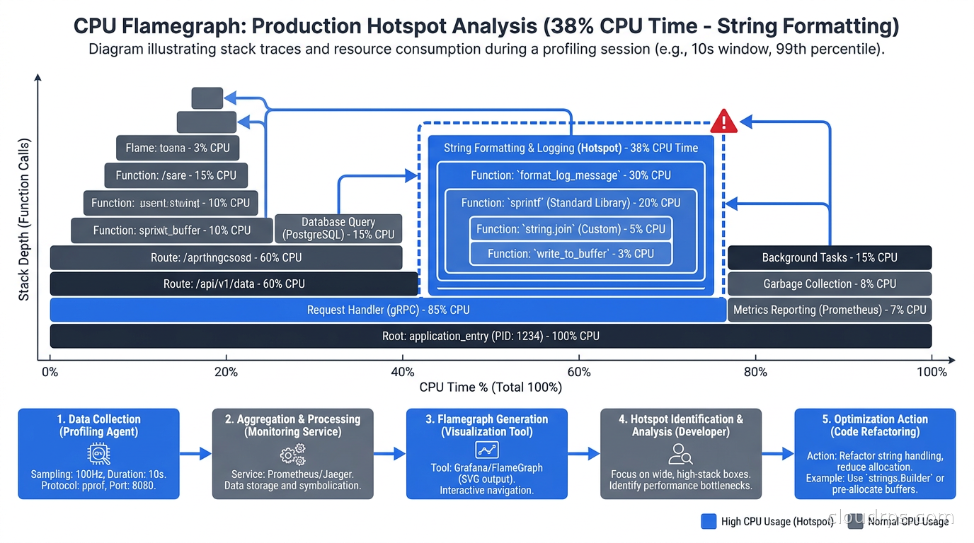
Sampling profilers interrupt the program at regular intervals (typically 100 times per second), capture the current call stack, and record it. Over thousands of samples, patterns emerge: if a function appears in 40% of samples, it is consuming approximately 40% of CPU time. The error margin is statistical, but for finding hot paths it is entirely sufficient.

Instrumentation-based profilers insert timing code into every function call. This gives exact measurements but imposes significant overhead and is generally not suitable for always-on production use. Some JVM profilers use this approach and the overhead shows.

eBPF profilers use the Linux kernel’s extended Berkeley Packet Filter subsystem to collect stack traces from the kernel without any changes to user-space code. This is the approach that makes language-agnostic, always-on profiling practical. The profiler runs in kernel space, interrupts processes at configurable intervals, and collects kernel and user-space stack traces together. You get a complete picture: your application code, the runtime, system calls, and kernel functions, all in one flamegraph.

The eBPF networking and observability deep dive covers how eBPF works at the kernel level. For profiling, the critical advantage is that eBPF profilers can profile anything running on the host without instrumentation or language-specific agents. One agent per node covers everything.

Reading Flamegraphs

The flamegraph is the visual format that makes profiling data comprehensible. Brendan Gregg at Netflix invented it specifically to solve the problem of interpreting hundreds of thousands of stack trace samples in a way humans can act on.

In a flamegraph:

• The x-axis represents cumulative time spent, not time of occurrence. Width equals percentage of samples where that function was on the stack.
• The y-axis represents the call stack depth, with root frames at the bottom and leaf functions at the top.
• Wide boxes near the top of the chart are your hotspots. Find the widest plateau and look directly below it to see the call chain that led there.
• Color is typically meaningless (random or by package) unless the tool uses it to encode something specific like package ownership or regression severity.

The mistake I see constantly: engineers look at the tall stacks and assume height is the problem. It is not. Height means deep call chains, which is normal. Width is where the time went.

Different profile types answer different questions:

• CPU profile: where is compute going?
• Heap/allocation profile: what is creating garbage collection pressure?
• Goroutine profile (Go): are there goroutine leaks? What are blocked goroutines waiting on?
• Mutex profile: where is lock contention hurting throughput?
• Block profile: what is blocking on I/O, channels, or system calls?

The allocation profile is frequently more revealing than the CPU profile. A service can have low CPU utilization but excessive GC pauses caused by a high allocation rate. Memory allocations that do not survive long enough to appear as heap usage still punish you with GC cycles.

The Tools: Pyroscope, Parca, and the Cloud Options

Grafana Pyroscope

Pyroscope started as an independent open-source project and is now fully integrated into the Grafana observability stack. As of 2026, it occupies the profile storage and query role alongside Loki (logs), Mimir (metrics), and Tempo (traces). The LGTM stack now effectively includes a fifth letter.

The cloud-native observability stack with Prometheus, Loki, Grafana, and Tempo covers the foundation most teams already run. Adding Pyroscope slots in alongside those components using the same Grafana data source model.

Pyroscope operates in three modes:

Pull mode via Grafana Alloy: The Alloy agent scrapes profiles from applications that expose a pprof-compatible HTTP endpoint, similar to how Prometheus scrapes metrics. Go’s standard library exposes pprof endpoints automatically once you import net/http/pprof. This is the easiest entry point for Go services.

Push mode via SDK: Applications use the Pyroscope SDK to push profiles to the Pyroscope server. Required for languages and runtimes that do not expose pprof-compatible endpoints. Available for Go, Python, Java, Ruby, Node.js, Rust, and .NET.

eBPF mode via Grafana Alloy: The Alloy agent runs an eBPF profiler that profiles all processes on the node without any application-side changes. This is the mode I recommend for greenfield deployments. You deploy one Alloy agent per node as a DaemonSet, and every container on that node gets profiled automatically. No SDK changes, no pprof endpoints, no per-service configuration.

For polyglot environments (multiple languages in one cluster), eBPF mode is the only practical option that covers everything without per-service instrumentation work.

Parca and Polar Signals

Parca is the open-source continuous profiler from Polar Signals, built by engineers who previously worked on Prometheus, Thanos, and other CNCF projects. It takes a different architectural approach: eBPF-only collection, with a purpose-built columnar storage engine optimized specifically for profile data query patterns.

The Parca Agent runs as a DaemonSet and automatically discovers all processes on each node. No SDKs, no application changes. The storage backend is designed around the query “show me the CPU profile for service X across all pods, aggregated and symbolized, for this time range.”

The feature that distinguishes Parca from Pyroscope is its profile diff capability. You can write a query that compares the CPU profile for version 1.4.2 against version 1.4.1, and Parca renders a differential flamegraph where regressions appear red and improvements appear blue. This version-aware comparison is genuinely powerful for catching performance regressions at deploy time.

Polar Signals offers a managed cloud backend if you want to avoid operating the storage layer yourself.

Google Cloud Profiler

Cloud Profiler is the managed option for GCP-native teams. You add a small initialization block to your application code and Cloud Profiler handles collection and storage. Supported languages include Go, Python, Java, and Node.js.

The operational simplicity is real: no infrastructure to run, no storage to manage, no scaling concerns. For teams that do not want to operate another stateful system, this is a reasonable starting point. The UI is less powerful than Pyroscope or Parca, and there is no eBPF mode or automatic discovery of uninstrumented services. But it works reliably and is dirt cheap at GCP pricing.

AWS CodeGuru Profiler

CodeGuru Profiler covers Java and Python on AWS. It integrates with CloudWatch and includes automatic anomaly detection: it flags when a function’s resource consumption changes significantly between releases, which is genuinely useful for catching regressions during a deployment window.

I have used it in Java microservice environments and found the anomaly detection practical. You configure it to compare against a baseline period and it emails you when something shifts. The scope is narrower than the open-source options, but the operational burden is essentially zero.

Deploying Continuous Profiling in Kubernetes

The practical deployment architecture for most Kubernetes environments:

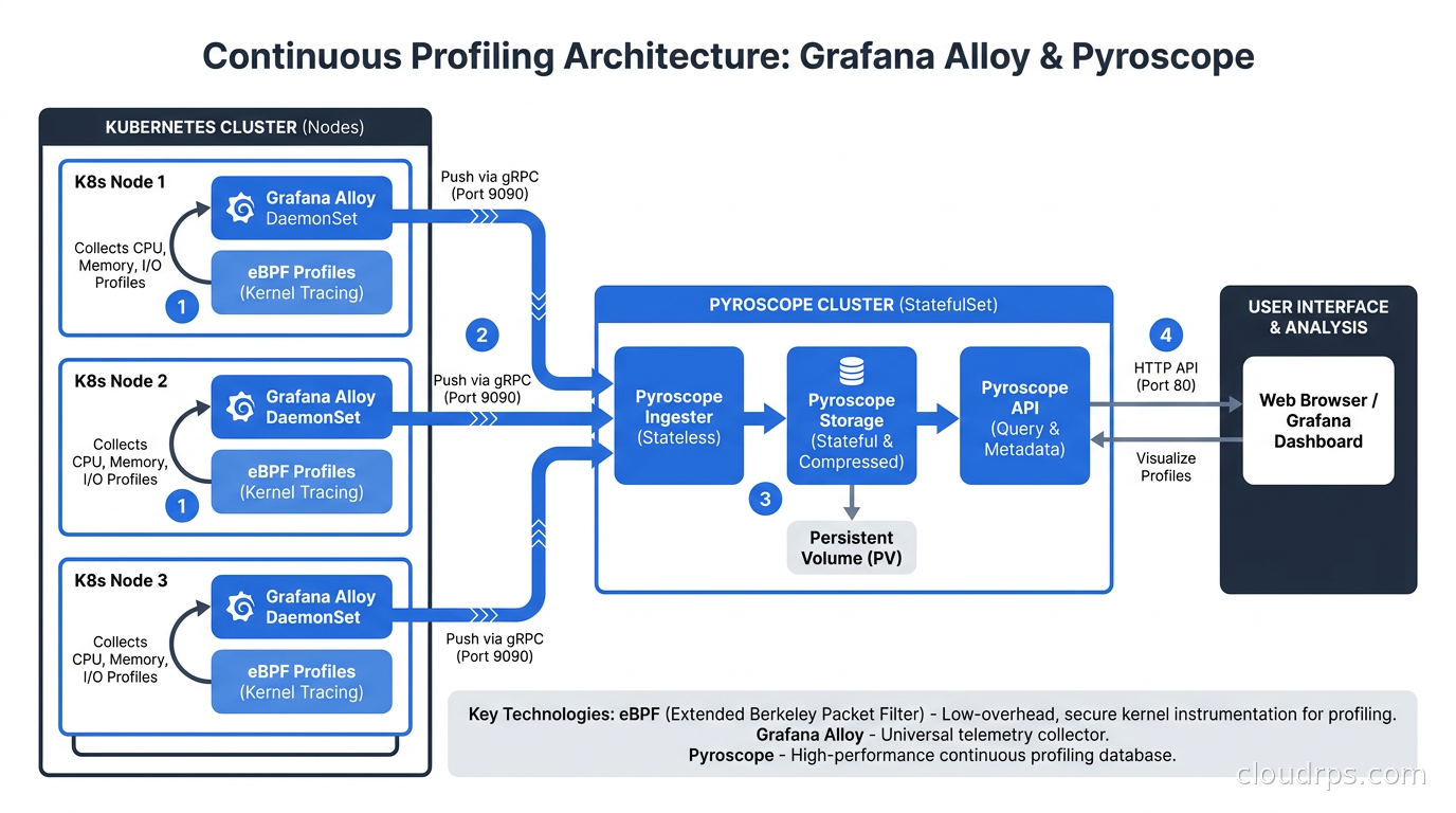
Step 1: Deploy Alloy as a DaemonSet with eBPF profiling enabled

The Alloy agent needs specific Linux capabilities to run the eBPF profiler. At minimum: SYS_ADMIN and SYS_PTRACE. Some environments also require SYS_BPF depending on kernel version. The agent also needs access to /sys and /sys/kernel/debug host paths.

A simplified Alloy configuration enabling eBPF profiling and sending to Pyroscope:

pyroscope.ebpf "default" {
  targets = discovery.kubernetes.pods.targets
  forward_to = [pyroscope.write.local.receiver]
}

pyroscope.write "local" {
  endpoint {
    url = "http://pyroscope.monitoring.svc.cluster.local:4040"
  }
}

The discovery component uses Kubernetes pod labels to automatically attach service name, namespace, and pod name as labels on every profile, so your flamegraphs are immediately filterable by service.

Step 2: Deploy Pyroscope

Pyroscope is available as a Helm chart. For a starting configuration, a single-node deployment with a 100GB PVC handles moderate-sized environments. Profile data compresses 5-10x, so 100GB of raw storage holds significantly more than the number suggests.

For high-availability deployments, Pyroscope supports a distributed mode analogous to Mimir’s microservices mode. Most teams starting out do not need this: single-node Pyroscope with a large PVC and regular backups is simpler and sufficient.

Step 3: Label everything

Label discipline with profiles is as important as with metrics. At minimum attach: service name, version, environment (prod/staging), and Kubernetes namespace. These labels are what let you ask “did CPU utilization increase when we rolled out version 1.5?” without guessing.

The version label is especially important. Pyroscope and Parca can both diff profiles between label values. Without a version label, you cannot compare v1.4 to v1.5 profiles.

Step 4: Add SDK instrumentation for interpreted languages

eBPF stack traces for Python, Ruby, and pre-JIT JVM code are often incomplete because the kernel cannot symbolize the interpreter’s internal frame structures. For these languages, the language-specific agent produces better results.

For Python: pip install pyroscope-io and a three-line initialization block. The Pyroscope Python agent uses py-spy under the hood, which handles CPython’s frame structure correctly.

For JVM languages: the async-profiler backend produces mixed-mode profiles that include both Java frames and native frames, giving you the complete picture including JVM internals.

Correlating Profiles with Traces and Metrics

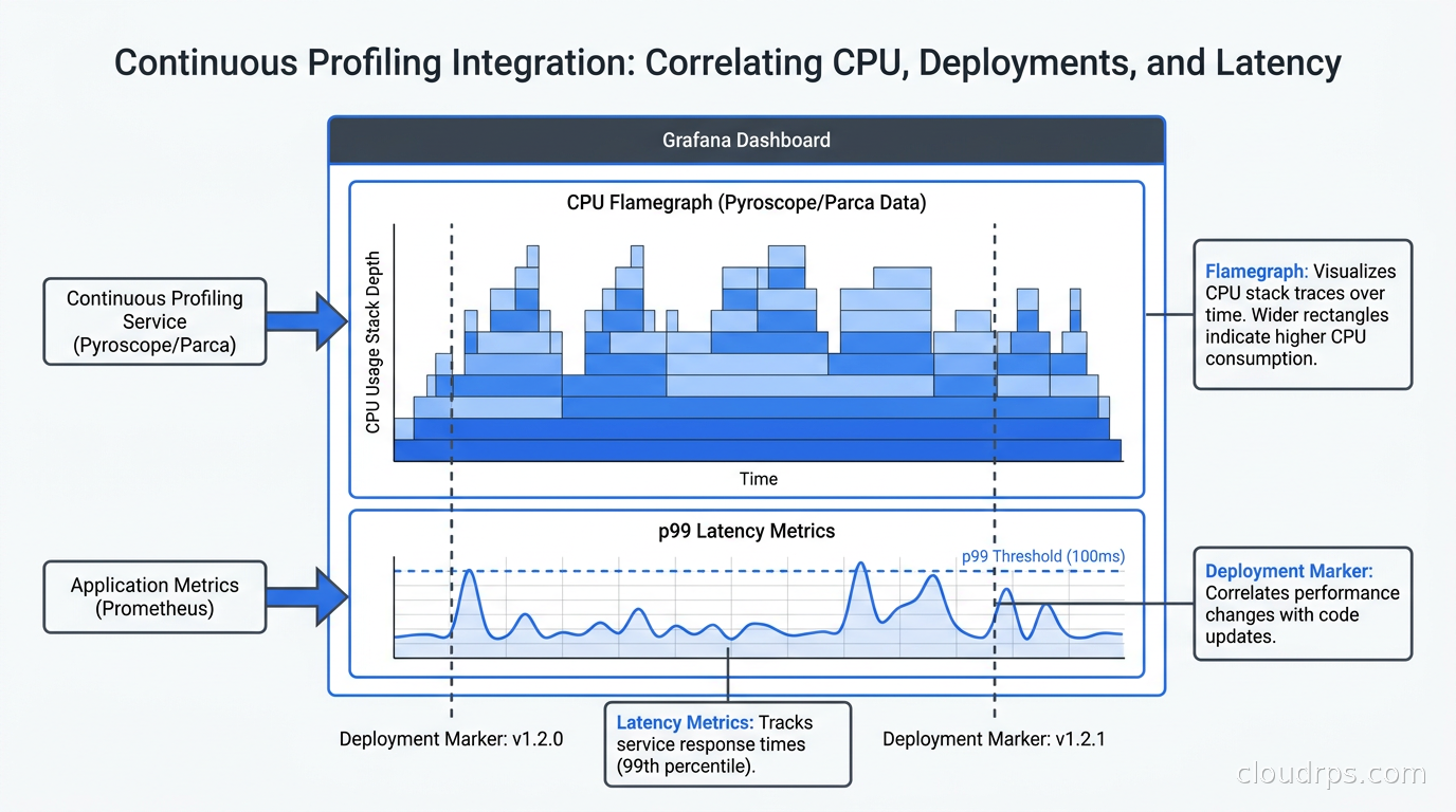
The real power of continuous profiling is correlation. When you see a latency spike in your distributed trace, you want to jump directly to the CPU profile for that service at that moment.

OpenTelemetry and distributed tracing provide the request-level context: which service was slow, which operations took time, which downstream calls added latency. Continuous profiling provides the code-level context: which function consumed the CPU, which allocator created the memory pressure. They answer different levels of “why was this slow.”

Grafana connects these signals through its explore view. Starting from a slow Tempo trace, you can click “profile” and Grafana fetches the Pyroscope data for the relevant service, time window, and Kubernetes pod. The connection works best when you use Grafana Alloy for all telemetry collection, because the agent can correlate trace IDs with profile collection windows.

This integration is still maturing. In practice, the time-window correlation (rather than exact trace ID correlation) is sufficient for most investigations: find the time when latency spiked in your metrics dashboard, then open the profile for that same window in Pyroscope.

Real-World Use Cases

Here are problems I have watched continuous profiling identify that would have taken weeks to find otherwise:

The invisible JSON tax: A Python service was spending 38% of its CPU in json.dumps(), serializing response objects that were immediately deserialized by the calling service. Both services had been written by different teams over two years. Switching to a binary serialization format cut CPU by 30% and allowed downsizing the instance type at the next capacity review.

The regex that rebuilt itself: A high-traffic Java service was compiling a Pattern.compile() on every request because a developer had moved initialization code out of a static block during a refactor, not realizing the implication. The pattern string was identical every time. The compilation showed as the widest node in the CPU flamegraph. Moving it back to a static field took five minutes.

The connection leak that hid in heap: Heap allocation profiles showed memory growing at a steady rate, surviving full GC cycles. The allocation flamegraph showed connection objects allocated in one path with no corresponding deallocation. A conditional branch was silently skipping defer conn.Close(). No metrics or traces would have surfaced this directly.

The O(n squared) lurker: A data processing service performed acceptably at small data sizes, so load tests passed. In production, as data grew, a loop-within-a-loop pattern became visible in CPU profiles as one inner function consuming a growing percentage of cycles. The profile history showed the trend: that function had grown from 5% of CPU six months ago to 45% today, directly correlated with data volume growth. Restructuring the lookup into a hash map fixed it.

Managing Overhead and Cost

Realistic overhead numbers for the common approaches:

• Go pprof at 100Hz sampling: 1-3% CPU
• eBPF profiling via Grafana Alloy: 1-5% CPU, minimal memory
• Java async-profiler: 1-3% CPU
• Python py-spy: 1-2% CPU

These are averages for typical production workloads. Services with extremely high call rates or many goroutines can push eBPF overhead higher. I recommend benchmarking in staging with production-representative traffic before enabling across the fleet.

Storage costs depend on fleet size and retention. A large cluster with 100 services and 1000 pods generates roughly 50-200GB of profile data per day before compression, and 10-40GB after. At object storage prices, this is inexpensive. The concern is more about the Pyroscope PVC growing unbounded if you do not configure retention.

Reasonable retention defaults:

• 7 days of full-resolution profile data
• 30 days of downsampled profiles (useful for deployment-over-deployment comparison)
• Permanent archives of profiles from incident windows (pull them to object storage manually or via a retention rule)

If your profiling backend is in a different region from your services, profile data transfer costs add up. See the cloud egress costs and architecture guide for how to reason about cross-region data movement. Colocate Pyroscope with the services it is profiling.

Integrating Profiling into Your SRE Practice

Continuous profiling changes the economics of performance work. Instead of reactive profiling (run a profiler when something is on fire), you build a historical record that enables proactive practices:

Pre-release performance gates: Compare CPU and memory profiles between the current release and the previous version before promoting to production. A 20% increase in allocation rate warrants investigation before the change ships. Tools like the Pyroscope API and Parca’s diff functionality make this automatable in your CI/CD pipeline.

Capacity planning accuracy: Profiles reveal whether CPU utilization is dominated by business logic, serialization, GC, or system calls. This changes how you forecast capacity requirements and which optimization efforts will actually move the needle. SLO and error budget management becomes more precise when you understand what CPU cycles are actually purchasing.

Incident post-mortems: Profile data from the incident window is the most honest record of what the service was doing. Pair it with the timeline from your metrics and traces for a complete picture.

Gradual regression detection: Performance that degrades 2% per week is invisible in metrics dashboards. With profile history you can compare this week’s CPU profile to three months ago and see which functions grew, correlated against the git history of what changed.

Getting Started Without Boiling the Ocean

My recommended path for teams starting from zero:

Week 1: Enable eBPF profiling on one service via Grafana Alloy without touching application code. Deploy a single-node Pyroscope instance with a 50GB PVC. Spend time learning to read flamegraphs and understanding what normal looks like for that service.

Week 2-3: Expand the DaemonSet to cover the full cluster. Add SDK-based profiling for Python or JVM services where eBPF stack traces are incomplete.

Month 2: Add version labels, configure Grafana to show profiles alongside metrics and traces, and train the team on the basic correlation workflow.

Quarter 2: Automate profile comparison in your deployment pipeline. Use the Pyroscope HTTP API or the Parca CLI to compare profiles between versions and fail the pipeline when CPU or allocation regressions exceed your threshold.

The monitoring and logging best practices article covers the foundational observability hygiene you need in place before layering profiling on top. If your metrics and logs are not clean, adding profiles will just give you more data to be confused by.

Conclusion

Continuous profiling is the observability signal that converts “something is slow” into “this specific function on this specific code path is the problem.” The tooling has matured: Grafana Pyroscope is production-ready and integrates naturally with the LGTM stack most teams already run; Parca offers compelling version-diff capabilities with stronger Prometheus alignment; managed cloud options from GCP and AWS reduce operational overhead for teams that prefer not to run another stateful backend.

The overhead is low enough (1-5% CPU) that the cost of not running profiling, measured in incident duration and engineering time, vastly exceeds the cost of running it. Deploy the DaemonSet, ship the backend, and give your team the ability to answer “where did the CPU go” with a flamegraph click rather than a two-week investigation.

That string formatter I mentioned at the start cost approximately 40,000 CPU-hours of wasted compute over six months before we found it. A Pyroscope deployment would have surfaced it on day one. The math on that one is not close.