DynamoDB in Production: Single-Table Design, GSI Overloading, and the Data Modeling Decisions That Actually Scale

Twenty years building cloud infrastructure has taught me that nothing separates senior engineers from everyone else faster than watching them try to use DynamoDB like a relational database. I have seen teams burn months on a data model that looked perfectly sensible on a whiteboard, then fell apart the moment it hit production load, because they applied PostgreSQL intuitions to a fundamentally different system.

DynamoDB is AWS’s fully managed key-value and document database. It handles massive scale with single-digit millisecond latency, scales horizontally without any operational intervention, and backs some of the highest-traffic systems at Amazon. It is also genuinely difficult to use correctly. The design decisions you make upfront determine whether your queries cost pennies or a fortune, and whether your schema will adapt to new access patterns or require an expensive remodel.

This is the DynamoDB guide I wish I had twenty years ago when I first modeled production data on it.

The Mental Model Shift

Start here before you touch a table or write a line of code.

In a relational database, you design your schema to represent your data, then write queries against it later. DynamoDB inverts this completely. You design your schema around your access patterns. Before you create a table, you need to know exactly how your application will read and write data. Every query that matters in production needs to be a first-class citizen in your data model.

This is not a limitation. It is a deliberate trade-off. DynamoDB can guarantee single-digit millisecond reads at any scale because it never needs to scan, sort, or join across arbitrary predicates. Every query on a well-designed DynamoDB table is a direct key lookup or a bounded range scan within a single item collection. The database does not need to think. That predictability is what makes it work at Amazon scale.

If your access patterns are unknown, or if you need ad-hoc querying and flexible analytics, DynamoDB is the wrong choice. More on that at the end. But if you have a well-understood set of access patterns that need consistent, low-latency performance under variable load, it is one of the most operationally simple databases available. Understanding where it fits in the SQL vs NoSQL landscape is the starting point for every DynamoDB evaluation.

Primary Keys: The Foundation Everything Builds On

Every DynamoDB item has a primary key. Two options exist:

A simple primary key uses just a partition key (hash key). Items are identified by a single attribute, like userId or orderId. Use this when you only ever look up items by their unique identifier.

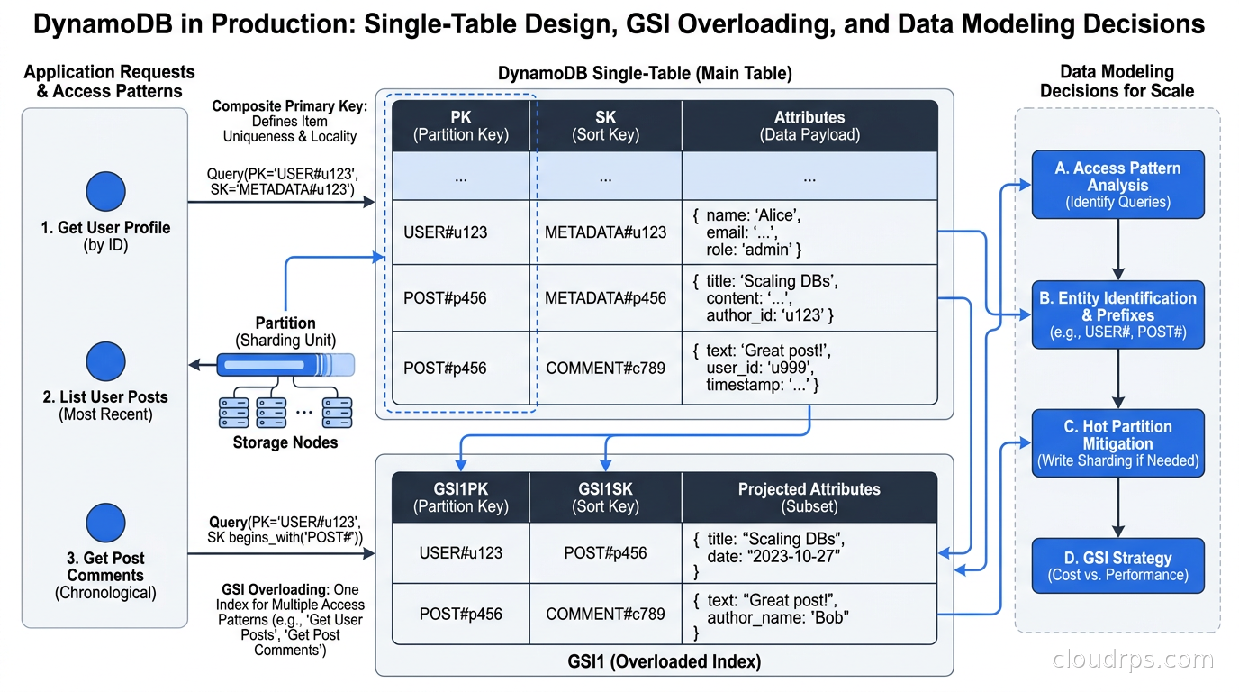
A composite primary key combines a partition key and a sort key. This is where DynamoDB gets interesting. All items sharing the same partition key form an item collection and are stored together physically, sorted by the sort key. This lets you model one-to-many relationships and retrieve multiple related items in a single request without multiple round trips.

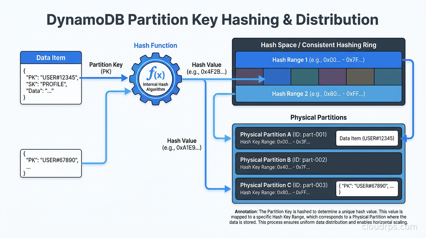
The partition key gets hashed and determines which physical partition stores the item. DynamoDB divides your table across partitions automatically, which is where your first major design decision lives.

Hot Partitions: The Classic Failure Mode

If your partition key values are not well-distributed, you will concentrate traffic on a small number of physical partitions while the rest sit idle. This is a hot partition, and it will cap your throughput and cause throttling errors even when your table has plenty of overall capacity.

I have seen this happen with user IDs on a table where a small number of highly active accounts generated the vast majority of traffic. The obvious fix, using a high-cardinality attribute like a UUID as the partition key, does not always solve the problem when you have celebrity accounts or viral content. For those cases, write sharding helps: append a random numeric suffix (like userId#0, userId#1, userId#2) to distribute writes across multiple partition keys, then scatter-gather reads across all shards.

The other hot partition trap is using a date as the partition key. All writes go to today’s partition while yesterday’s partitions sit cold. For time-series data, model the time component as a sort key instead, and use a high-cardinality attribute as the partition key to ensure even distribution across partitions.

Single-Table Design

AWS’s own documentation recommends keeping the number of tables per application to a minimum. In the majority of cases, AWS recommends a single table.

This seems counterintuitive coming from a relational background. In PostgreSQL, you have a users table, an orders table, and an order_items table. In DynamoDB, all three might live in one table, distinguished by their key structure and an item type attribute.

Here is what single-table design looks like in practice for an e-commerce application:

For a user item: partition key = USER#u123, sort key = PROFILE For a user’s order: partition key = USER#u123, sort key = ORDER#2026-10-01#o789 For an order item: partition key = ORDER#o789, sort key = ITEM#sku-456

All of a user’s orders live in the same item collection as the user record, sorted chronologically by the sort key. A single query with a begins_with sort key condition retrieves a user and all their orders from the same physical partition in one round trip. No joins. No secondary lookups.

The alternative, multiple tables, forces multiple network calls to fetch related data, increases operational overhead, and prevents you from leveraging DynamoDB’s item collection model. For most applications, single-table design is the correct default.

Where Single-Table Design Creates Problems

Single-table is not universally correct. If you are building a multi-tenant SaaS platform where tenants have radically different access patterns, forcing everything into one table can make the schema difficult to reason about as the team grows. Some teams draw the line at one table per microservice rather than one table per application, which gives you team isolation without the cross-service join problem. The right call depends on team size, schema complexity, and the organizational cost of managing multiple tables.

Global Secondary Indexes and Overloading

DynamoDB’s Global Secondary Indexes (GSIs) let you define alternate key schemes for the same data, enabling access patterns that the primary key cannot serve. You can add up to 20 GSIs per table, though most well-designed tables need fewer than five.

GSI overloading is the pattern that makes single-table design practical at scale. Instead of creating a separate index per entity type, you define generic GSI key attributes like GSI1PK and GSI1SK, then populate them with different values depending on the item type. The GSI projects only the items where those attributes are set, giving you a filtered view of the table by entity type.

For example, in a single-table application:

• On user items: GSI1PK = EMAIL#user@example.com, enabling lookup by email address
• On order items: GSI1PK = STATUS#pending, enabling retrieval of all pending orders
• On product items: GSI1PK = CATEGORY#electronics, enabling browsing by category

One GSI serves three completely different access patterns on three different entity types. This is GSI overloading, and it is how you avoid burning through your 20-GSI limit with a separate index per entity.

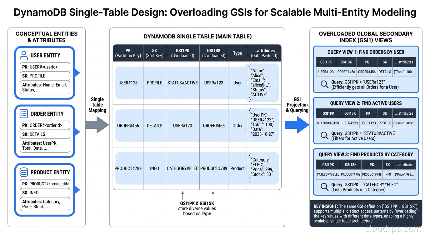
Sparse indexes complement overloading. DynamoDB only adds an item to a GSI when that item has the indexed attributes set. Leave GSI1PK and GSI1SK off items that do not need that access pattern, and the GSI stays small. A table with ten million user items and a hundred thousand pending orders can have a GSI containing only those hundred thousand orders, making scans of that GSI cheap and fast.

Capacity Modes and Cost Reality

DynamoDB offers two capacity modes: provisioned and on-demand.

In provisioned mode, you set read capacity unit (RCU) and write capacity unit (WCU) limits. The database will not exceed those limits. One RCU handles one strongly consistent read per second for items up to 4KB, or two eventually consistent reads. One WCU handles one write per second for items up to 1KB. Auto scaling adjusts capacity within defined bounds, but you pay for the capacity you provision whether or not traffic uses it.

On-demand mode scales automatically with no capacity planning required. You pay per request. In March 2025, AWS cut on-demand throughput prices by 50%. The current pricing in us-east-1 is $1.25 per million write request units and $0.25 per million read request units (verify the current rate at aws.amazon.com/dynamodb/pricing before making cost projections, as these rates are subject to change).

Provisioned capacity is cheaper for steady, predictable traffic. On-demand suits spiky workloads, new applications where traffic patterns are unknown, or services with infrequent bursts. A common approach is to start on on-demand, watch usage metrics for several weeks, then switch to provisioned auto scaling with reserved capacity once patterns stabilize. Reserved capacity offers significant savings on top of provisioned: AWS offers one-year and three-year reserved capacity terms with substantial discounts.

Item size has an outsized effect on cost. DynamoDB rounds each write up to the nearest 1KB and each read up to the nearest 4KB. Storing large JSON blobs directly in items will multiply your costs. Keep items lean. Store large payloads in S3 and maintain only a reference key in DynamoDB.

Transactions

DynamoDB supports ACID transactions via TransactWriteItems and TransactGetItems. You can atomically write or read up to 100 items across one or more tables in a single call. Each transactional operation consumes 2x the normal capacity units.

Reserve transactions for operations that genuinely require atomicity across multiple items, such as a financial transfer, an inventory reservation that must check and update stock simultaneously, or a business-critical state machine transition. The 2x capacity overhead adds up quickly if you use transactions as a default rather than an exception.

For most operations, lean on DynamoDB’s native item-level atomicity. Conditional writes let you update an item only if a specified condition is met, which covers many common use cases without transactional overhead. Understanding how ACID properties work across database families helps clarify when DynamoDB’s transaction model is sufficient and when a relational database would be less friction. The consistency trade-offs involved also relate directly to the CAP theorem.

DynamoDB Streams and Change Data Capture

DynamoDB Streams captures a time-ordered sequence of item-level changes in your table. Each stream record contains the item’s old and new images along with a sequence number. Records are retained for 24 hours.

The primary use case is triggering Lambda functions on table changes. Streams and Lambda together power a large fraction of DynamoDB-backed event-driven architectures on AWS. An order creation triggers an email confirmation. An inventory drop below threshold triggers a reorder workflow. A user profile update propagates to a search index.

Streams also underpin cross-region replication in Global Tables and enable exporting change data to analytics pipelines. If you are familiar with change data capture patterns using Debezium and Kafka for relational databases, DynamoDB Streams provides similar capability without additional tooling, though with a 24-hour retention limit rather than Kafka’s configurable retention.

One critical operational point: Lambda consumers process Streams records in shard order. A Lambda that throws an unhandled error will block the shard until the error resolves or the record expires (24 hours). Model your Lambda functions to be idempotent, implement dead-letter queues for persistently failing records, and set appropriate maximum retry configurations.

DynamoDB Accelerator (DAX)

For workloads that need microsecond read latency instead of millisecond, DynamoDB Accelerator (DAX) provides an in-memory caching layer with a DynamoDB-compatible API. Your application points at the DAX cluster endpoint. Cache hits return in microseconds. Cache misses fall through to DynamoDB, populate the cache, and return normally.

DAX works best for read-heavy workloads with repetitive reads of the same items: product catalogs, leaderboards, configuration tables, frequently accessed reference data. It is less useful for workloads where data changes frequently or where per-user data is rarely reread.

Compared to using Redis or Valkey as a separate caching layer, DAX has two advantages: it integrates directly with the DynamoDB API (no separate cache client or invalidation logic in application code) and it maintains write-through consistency automatically. Redis offers more flexibility for complex caching strategies and works across multiple data sources, but you own the invalidation logic. For applications already committed to DynamoDB where read performance is the bottleneck, DAX is the lower-complexity path.

Global Tables and Multi-Region Strong Consistency

DynamoDB Global Tables provide active-active multi-region replication. Writes to any region replicate to all other participating regions automatically. This enables multi-region architectures with low read latency globally and regional failover capability without operator intervention.

The traditional limitation was eventual consistency across regions for global reads. In July 2025, AWS introduced Multi-Region Strong Consistency (MRSC) for Global Tables. Per AWS’s documentation, MRSC allows strongly consistent reads across regions with a Recovery Point Objective of zero during regional failures. This changes the viability of Global Tables for a class of applications, including financial systems and inventory management, that previously could not accept the eventual consistency trade-off.

Before MRSC, strongly consistent reads in Global Tables were limited to the local region. MRSC extends that guarantee across participating regions.

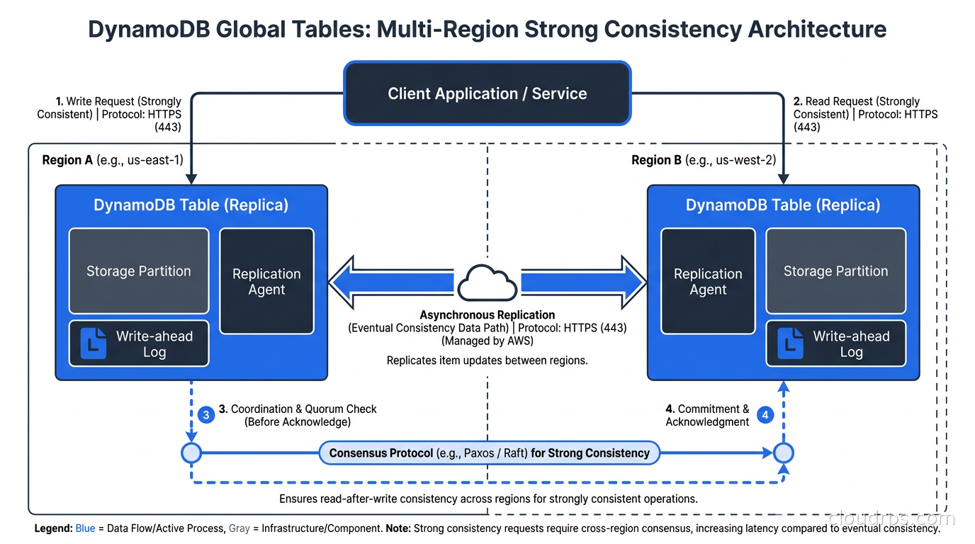
Global Tables fit naturally into multi-region active-active architecture patterns. For teams evaluating global database options, the comparison against distributed SQL databases like CockroachDB and Spanner is worth working through carefully. Distributed SQL offers globally distributed ACID transactions natively; DynamoDB Global Tables with MRSC provides strongly consistent reads but still applies last-writer-wins semantics for conflicting concurrent writes across regions. For workloads where cross-region write conflicts are common, distributed SQL may be a better architectural fit.

Vector Search: The August 2026 Addition

In August 2026, AWS made vector search for DynamoDB generally available. You can now store vector embeddings alongside your existing DynamoDB attributes and run similarity searches directly against the table, without a separate vector store.

This matters for RAG architectures where DynamoDB is already the primary data store. Previously, you needed a separate vector database for embedding-based retrieval, then a second lookup in DynamoDB to hydrate the full item. Native vector search collocates the embeddings with the items they describe, reducing architectural complexity and the latency of a cross-system round trip.

The feature supports vectors up to 4096 dimensions with multiple distance functions. Compare this against dedicated vector stores when evaluating: pgvector for PostgreSQL-native vector search and Amazon S3 Vectors for high-volume, cost-optimized vector storage at scale. DynamoDB vector search is the right choice when your application already uses DynamoDB as its primary store and needs similarity search as a secondary access pattern. If vector similarity search is your primary workload, purpose-built vector databases or S3 Vectors will give you better cost efficiency and richer query capabilities.

Hard Limits That Catch Teams Off Guard

DynamoDB has limits that matter in production:

Item size is capped at 400KB. Enough for most items, but if you are trying to store large documents or serialized objects, you need to store the payload in S3 and maintain a reference in DynamoDB.

Item collections, meaning all items sharing a partition key across the base table and all local secondary indexes, are capped at 10GB. Hitting this limit causes write rejections. Tables with local secondary indexes need active monitoring of per-partition item collection sizes. CloudWatch Contributor Insights surfaces partition-level metrics that make this visible before it becomes a user-facing problem.

DynamoDB limits vary by account and region: there are limits on the number of tables per account, on the number of concurrent GSI creations, and on the maximum item count for batch operations. The authoritative list is in the AWS DynamoDB Limits documentation, and it changes with service updates.

The maximum item count for TransactWriteItems is 100. For bulk loading, use BatchWriteItem instead, which supports up to 25 items per call, is not atomic, and does not consume 2x capacity. For large initial data migrations, PartiQL batch inserts or DynamoDB’s Import from S3 feature are more efficient than SDK batch writes.

When DynamoDB Is the Wrong Choice

I want to be direct here, because I have seen too many teams choose DynamoDB because it is AWS’s flagship NoSQL database, then spend months fighting its constraints.

DynamoDB is the wrong choice when your access patterns are unknown or evolving rapidly. The access-pattern-first design philosophy means that adding a new access pattern later may require a new GSI or a data model restructure. Early-stage products where requirements change frequently pay a high tax.

It is the wrong choice for complex analytics. Table scans are expensive, and filtering by non-key attributes is slow and costly. For anything analytics-adjacent, purpose-built OLAP databases serve you far better.

It is frequently a poor fit for complex transactional workflows involving many interdependent items. The 100-item transaction limit and 2x capacity cost of transactions add up quickly in systems with rich domain logic.

And it is often the wrong choice when PostgreSQL is right. A managed PostgreSQL instance with appropriate indexing strategies handles the vast majority of database workloads with much more flexible query capabilities, a richer ecosystem, and a lower cost of schema change. The operational simplicity of DynamoDB is real, but “no migrations” comes at the price of rigorous upfront modeling that punishes mistakes more harshly than relational databases do.

A Production Checklist

Before choosing DynamoDB for a new service:

Write down every access pattern the application requires before touching any API. Not the nice-to-haves. Every required production query. Verify that each one maps to a primary key lookup, a sort key range query, or a GSI lookup. If anything does not map cleanly, rethink the choice of database.

Choose partition keys with high cardinality and uniform access distribution. Load-test with a traffic distribution that reflects production reality, not uniform random traffic.

Default to single-table design unless you have a compelling reason otherwise. Start on on-demand capacity, profile real usage for a few weeks, then evaluate provisioned auto scaling with reserved capacity once traffic patterns stabilize.

Enable DynamoDB Streams from the start if you anticipate needing CDC, replication, or event-driven integrations later. Adding streams retroactively is safe, but retrofitting event consumers mid-launch is painful.

Set up per-partition-key metrics via CloudWatch Contributor Insights from day one. Hot partition problems are invisible in aggregate metrics until they cause user-facing throttling.

DynamoDB rewards upfront discipline and punishes corner-cutting more than almost any other database. Teams that take the time to model access patterns carefully build systems that are both extremely performant and remarkably operationally quiet. Teams that treat it as a schemaless document store with a JSON API are in for a difficult time.