GraphRAG in Production: Why Knowledge Graphs Beat Vector Search for Complex Enterprise Queries

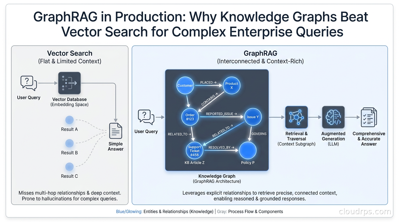
I have been building retrieval systems for twenty years, first for search engines, then for recommendation systems, and for the last several years for enterprise AI applications. Standard RAG felt like a major breakthrough when it landed: stop trying to squeeze the world into a context window; instead, pull in the relevant chunks at query time. That works beautifully for a narrow class of problems. Then I started hitting the wall that everyone eventually hits: queries where the answer exists only across five or six connected documents, none of which individually contains the answer. Your vector search retrieves three of the six. The LLM hallucinates the missing links. The business user loses trust in the system. You spend three weeks tuning chunk sizes and rerankers and gain back maybe ten percent of accuracy. I have seen this cycle play out at every organization that took RAG seriously.

GraphRAG exists because that wall is real. It is not a failure of reranking strategy or embedding model choice. It is a structural limitation of treating knowledge as a bag of semantically similar chunks. Knowledge is not a bag. Knowledge is a graph.

What Vector RAG Actually Gets Wrong

To understand why GraphRAG matters, you need to be clear about what vector RAG optimizes for. When you embed a chunk and store it, you are encoding “what does this passage talk about” into a high-dimensional point. When a query comes in, you find the nearest points. That works when the answer lives in a single passage or in a few passages that are semantically close to the question.

It fails on multi-hop questions: “Which of our suppliers have contracts that share a renewal date with any of our top-ten customers by revenue, and what is the combined exposure?” No single chunk answers that question. The answer requires traversing relationships: supplier contracts link to renewal dates, customer records link to revenue rankings, some dates overlap. Vector search will surface the chunks that mention suppliers and contract renewal dates and revenue, but it cannot traverse the structural connection between them. The LLM gets three puzzle pieces from a five-piece puzzle and guesses the rest.

The other failure mode is global synthesis: “What are the recurring themes in all incident reports from last quarter?” You cannot retrieve a representative sample of all incident reports by similarity to the question, because there are hundreds of reports and no single query captures all their themes. Standard RAG picks the most similar ones and misses the long tail. GraphRAG builds a community structure over all the data at indexing time, so global queries have pre-computed answers to draw from.

The GraphRAG Architecture

Microsoft Research released the original GraphRAG paper in 2024, and since then the ecosystem has matured considerably. The core architecture has two major phases: indexing and retrieval.

The Indexing Pipeline

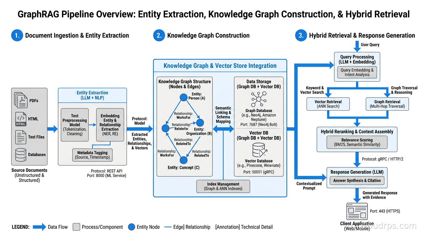
During indexing, every source document is chunked and sent through an LLM-driven extraction process. The LLM reads each chunk and returns structured data: entities (people, organizations, systems, concepts, locations) and the relationships between them. That extraction data feeds into a graph store. The system then runs a community detection algorithm, typically Leiden or Louvain, to cluster closely related entities into communities, and runs another LLM pass to generate a hierarchical summary for each community level.

This is where the cost conversation has to happen honestly. Entity and relationship extraction requires multiple LLM calls per document chunk. The exact count depends on your implementation, but the multiple-pass nature means GraphRAG indexing is substantially more expensive than pure embedding approaches. Microsoft’s original implementation using GPT-4o can consume tens of thousands of tokens per document, while leaner alternatives like LightRAG use a different architecture that reduces per-document token consumption significantly. I will come back to the trade-offs in the tooling section. The point is: you are making an architectural bet that the retrieval quality improvement justifies a meaningfully higher indexing cost. For enterprise knowledge bases queried thousands of times per day, it usually does. For a documentation set queried fifty times per week, it might not.

The Retrieval Layer

Query time in GraphRAG has two modes: local and global. Local queries target specific entities in the graph; the retriever starts from the entities most relevant to the query and walks the graph to collect neighboring context before generating the answer. Global queries use the pre-computed community summaries; rather than walking the live graph, the system retrieves the relevant community summaries and synthesizes across them. Global mode is what enables the “summarize all incident reports” class of queries.

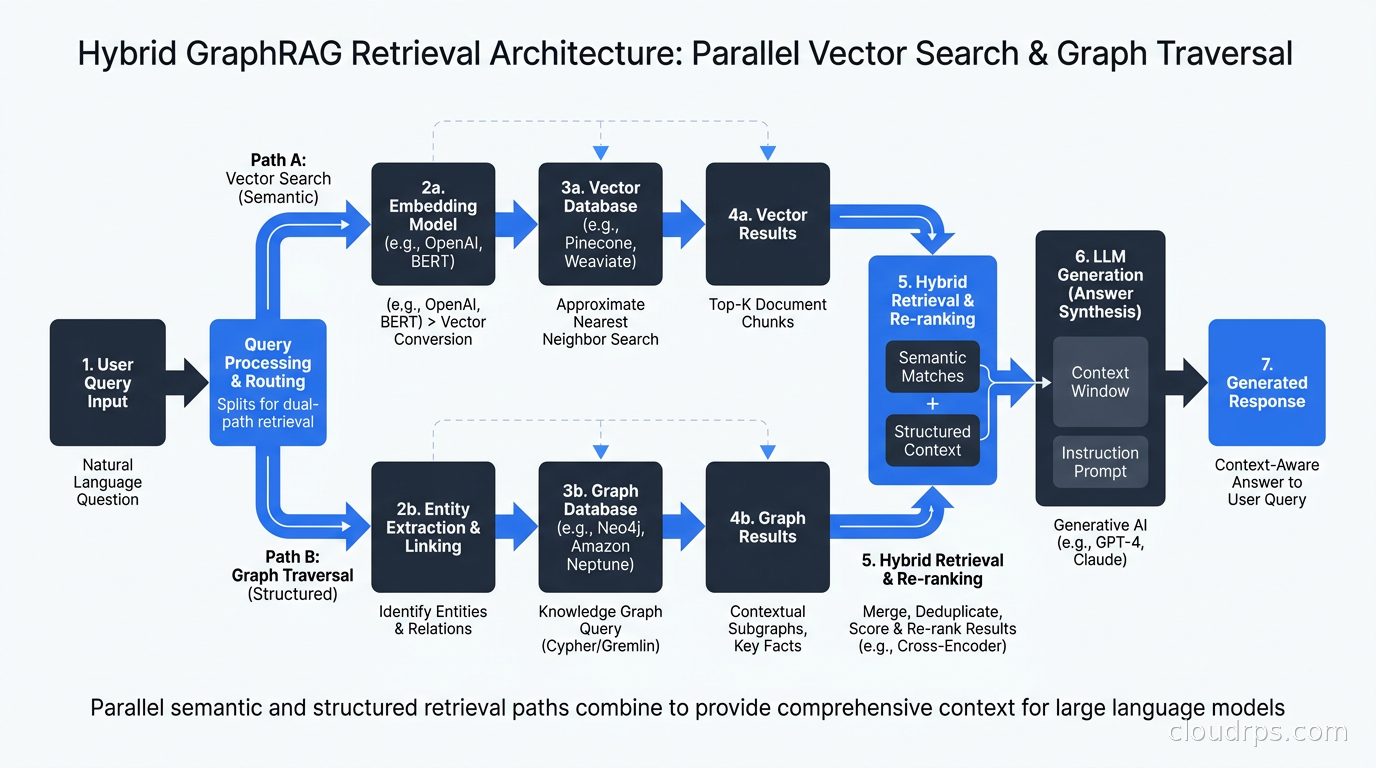
A production implementation typically augments both with vector search on the original chunks, so you get the graph-guided context plus the verbatim passages that contain supporting evidence. This hybrid retrieval pattern, running vector search and graph traversal in parallel and fusing the results before the final generation pass, delivers the best accuracy and is what mature production deployments look like.

Choosing a Graph Backend

Three main options exist for the graph store in a GraphRAG stack, and the choice matters more than it might seem.

Neo4j

Neo4j is the most mature and the most widely documented option. Microsoft’s open-source GraphRAG library has native Neo4j integration, and the community has extensive examples for LangChain and LlamaIndex pipelines on top of it. Neo4j runs on Kubernetes (with a Helm chart), is available on GCP Marketplace, and has a well-understood operational model.

The trade-off is resource consumption. Neo4j is a Java-based system with significant heap requirements, and for large knowledge graphs the memory footprint can be substantial. You also need to think about licensing: Neo4j Community Edition is open source under GPLv3, but Enterprise features required for production, such as clustering, role-based access control, and hot backups, require a commercial license. On AWS, you are typically running Neo4j on EC2 or EKS yourself; there is no managed service.

For existing teams with graph database experience, Neo4j is probably the lowest-friction choice. The Cypher query language is expressive, the tooling ecosystem is rich, and the documentation for GraphRAG use cases has improved dramatically over the past two years.

FalkorDB

FalkorDB is the spiritual successor to RedisGraph and was purpose-designed for GraphRAG workloads. It represents the graph as sparse adjacency matrices and executes queries as GraphBLAS linear algebra operations rather than pointer-chasing traversal. The architecture benchmarks claim substantial latency and memory improvements over Neo4j for GraphRAG-specific access patterns. FalkorDB publishes results from GraphRAG-Bench, an ICLR 2026 benchmark, that show their stack meaningfully outperforming baseline vector RAG on overall score.

One thing to flag clearly: FalkorDB’s license is SSPL, the same license Redis used before the BSL switch, and SSPL is not considered an OSI-approved open-source license. If your organization has policies about SSPL software, check before building on it. The managed cloud offering handles operations, but the licensing question is real.

Amazon Neptune

For teams already running on AWS with strict data residency requirements or complex IAM integration needs, Amazon Neptune is worth considering. Neptune is a fully managed graph database that supports both property graphs (Gremlin, openCypher) and RDF (SPARQL). You get Multi-AZ, automated backups, and native integration with AWS security controls. The trade-off is cost: Neptune is meaningfully more expensive at equivalent query volumes than self-hosted alternatives, and there is less published guidance on GraphRAG-specific access patterns compared to Neo4j. The AWS blog has an article on improving RAG accuracy with GraphRAG that covers Neptune integration patterns, which is worth reading if you are going the AWS-native route.

For most greenfield enterprise deployments, I recommend starting with Neo4j on Kubernetes unless you have specific reasons to prefer a different approach. The ecosystem maturity and available documentation are worth something real, especially for a team building its first knowledge graph pipeline.

The LightRAG Alternative

If you read the cost analysis for Microsoft’s GraphRAG implementation and felt your stomach drop, LightRAG deserves attention. LightRAG, introduced in late 2024, takes a different approach to knowledge graph construction: instead of extracting exhaustive entity-relationship triples from every chunk, it focuses on a smaller set of high-value entities and uses a dual-level retrieval strategy combining local and global modes. Per-document token consumption is substantially lower.

The accuracy trade-off depends on your corpus. LightRAG performs well on corpora where the entity graph is relatively sparse and you mostly need single-hop or two-hop reasoning. On complex enterprise datasets with dense relationship networks, the full Microsoft GraphRAG approach tends to win on multi-hop accuracy. The choice is not purely theoretical: you can prototype both approaches against a representative sample of your actual query distribution and measure before committing.

I have run this comparison twice in the past year. One project was a large compliance document corpus where most questions required only single-hop lookups; LightRAG delivered comparable accuracy at a fraction of the indexing cost. The other was a technical system dependency knowledge base where questions routinely required three and four hop traversals across service ownership chains; there, the full extraction approach justified its cost significantly.

Production Infrastructure Patterns

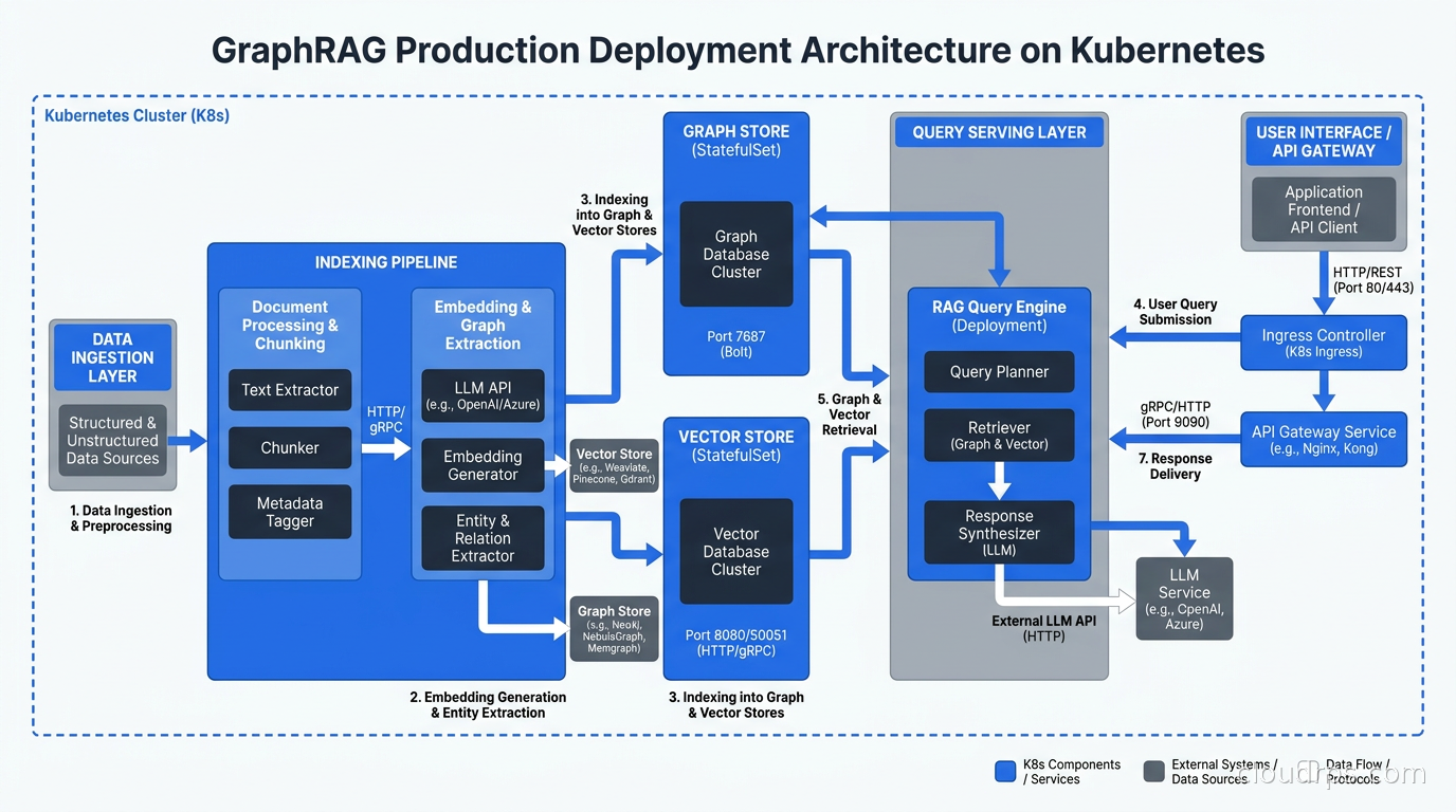
Deploying GraphRAG at enterprise scale involves more moving parts than a standard vector RAG stack. Here is the infrastructure pattern I have converged on for production.

Indexing as an Async Pipeline

Never run GraphRAG indexing synchronously at document upload time. The LLM extraction passes take non-trivial wall-clock time even with parallelism. Instead, use an event-driven pipeline: documents land in object storage, a message queue event triggers an indexing worker, the worker runs the extraction pipeline, and updates the graph store asynchronously. This lets you control throughput, retry on failures, and scale indexing workers independently from query serving.

The graph update problem deserves attention. Unlike a vector store where you can upsert a chunk independently, a knowledge graph has shared entities. When document A and document B both mention the same person, the graph has one node for that person with edges from both documents. When document A changes, you need to update that shared node’s context. GraphRAG libraries are still maturing their incremental update support; some teams avoid the problem by versioning the entire graph and rebuilding on major corpus changes. For frequently updated corpora this is expensive; for mostly-static enterprise knowledge bases, periodic full rebuilds are operationally simpler than incremental patching.

Serving Layer

The query path is latency-sensitive and needs to be separate from the indexing pipeline. For a production stack, I run the retrieval API as a stateless service that talks to both the graph store and the vector store, with the graph store being the component that requires most careful capacity planning.

For Neo4j, the read replica pattern is important for query throughput. Write your graph updates to the primary; route retrieval queries to read replicas. The number of replicas you need depends on your query volume and query complexity. Simple local queries with short traversals are fast; global queries that scan community summaries can be much slower depending on graph size and community structure. Instrument query latency distributions by query type from day one. The observability patterns from the LLM tracing guide apply directly here; add graph traversal time as a separate span in your traces.

Caching is surprisingly effective for GraphRAG workloads. Enterprise users tend to ask variations of the same questions repeatedly. A semantic cache in front of the retrieval layer, the same pattern described in the AI gateway architecture article, can capture a significant fraction of queries without hitting the graph at all. The key difference from standard RAG caching is that you want to cache at the level of the final response, not the retrieved context, because the graph traversal itself is the expensive step.

Storage Sizing

A common question is how large the knowledge graph becomes relative to the source corpus. There is no universal ratio; it depends heavily on entity density in your documents. Technical documentation tends to produce compact graphs. Legal documents and financial reports tend to produce dense graphs with many entity mentions. As a rough mental model: expect the graph store to be smaller than the original document corpus by size, but require more memory for efficient query execution than you would allocate for an equivalent-sized relational database.

The vector store for the chunk embeddings runs alongside the graph store. PostgreSQL with pgvector handles most production scales before you need to reach for a dedicated vector database. You want both systems on low-latency storage, ideally in the same availability zone as your query serving layer to minimize cross-AZ latency.

Cost Modeling Before You Commit

Before you build, model the cost honestly. The bill has three parts.

First, indexing cost. This is dominated by LLM API calls. Take a representative sample of your corpus, run the extraction pipeline against it, measure actual token consumption per document, and multiply by your corpus size. If you are using a hosted model like GPT-4o or Claude, the per-token rates are public. If you are running local inference, factor in the GPU time for the extraction passes. Do this before building the full pipeline; the number sometimes surprises people.

Second, graph store cost. Neo4j Enterprise licensing is non-trivial if your data requires it. Self-hosted on Kubernetes adds operational overhead. If you are using Neptune, the managed service cost has predictable pricing tiers but can be higher than you expect at volume. FalkorDB Cloud has its own pricing structure.

Third, ongoing re-indexing. Corpora change. If you maintain a GraphRAG index over a document set that changes weekly, you need a plan for incremental updates or periodic rebuilds and a budget for the associated LLM calls.

The AI FinOps framework applies to GraphRAG workloads just as it does to inference costs: understand your cost drivers per request, understand your usage patterns, and build controls before costs scale unexpectedly.

When GraphRAG Is Overkill

I want to be honest about when not to use GraphRAG. If your queries are primarily single-hop (“find me documents about X”), standard vector RAG with a good reranker covers most of the gap at a fraction of the infrastructure complexity. If your corpus is small enough that the entire thing fits in a long context window with room to spare, direct context stuffing can outperform both RAG approaches for certain query patterns.

GraphRAG earns its complexity when your corpus is large enough that full-context approaches are not viable, when queries require reasoning across multiple documents or entities, and when hallucination on cross-document synthesis is causing real business problems. That describes a lot of enterprise knowledge management and compliance use cases. It describes a subset of product use cases.

The RAG architecture production guide has a good decision framework for the basic vs. advanced RAG choice; GraphRAG fits into the upper end of that framework, appropriate when the advanced approaches are still not solving the multi-hop problem.

Connecting GraphRAG to AI Agents

The most interesting production use case emerging in 2026 is GraphRAG as the memory and knowledge layer for autonomous AI agents. An agent that needs to reason about entity relationships, organizational structures, or system dependencies can query the knowledge graph as a tool call, get structured graph data back, and reason over it far more reliably than if it were searching through flat document chunks.

This connects directly to the context engineering work described in context engineering for production AI agents: instead of stuffing context by similarity, you navigate it by relationship. The agent knows that answering a question about supplier risk requires traversing the supplier-to-contract-to-renewal-date-to-financial-exposure path; it issues graph queries to walk that path and assembles the context from structured results rather than from fuzzy semantic nearest-neighbors.

I expect this pattern to become standard architecture for enterprise AI applications over the next two years. The combination of a well-maintained knowledge graph with an agent layer that knows how to query it is more reliable for structured reasoning tasks than anything a pure vector approach can offer, and the infrastructure to support it is now genuinely production-ready.

Monitoring GraphRAG in Production

GraphRAG adds a few monitoring concerns beyond standard RAG. Track these metrics.

Graph freshness: how old is the most recently indexed document, and what fraction of the corpus has been indexed. Staleness in the knowledge graph is a source of subtle accuracy degradation that is easy to miss.

Entity extraction quality: sample your extraction outputs periodically and manually review them. LLM-based extraction is not perfect; entities get merged incorrectly, relationships get mislabeled, and the quality degrades on domain-specific technical content if your extraction prompts are not tuned for your corpus. Catching this early saves you from debugging mysterious accuracy regressions later.

Graph query latency by type: local queries and global queries have very different latency profiles. Segment them in your metrics. A spike in global query latency might mean your community summaries need rebuilding after a major corpus update, not that your serving infrastructure is undersized.

Response accuracy on your golden dataset: the LLM evaluation frameworks all support RAG evaluation, and the retrieval quality metrics they provide (context precision, context recall) apply directly to GraphRAG. Build a curated set of multi-hop questions with known answers for your specific knowledge domain and run it on every deployment.

The Bottom Line

Twenty years of building retrieval systems has taught me that the right tool depends on the shape of your queries. If your users are asking questions that require reasoning across multiple connected facts, standard vector RAG is not going to get you there no matter how much you tune it. GraphRAG solves a real problem by treating knowledge as a graph rather than a bag of chunks, and the production ecosystem has matured enough that you can build on it without pioneering entirely new territory.

The infrastructure investment is real: more complex pipeline, higher indexing costs, an additional stateful store to operate. Justify it with a concrete accuracy comparison on your specific query distribution, not on general benchmarks. When the use case fits, the improvement in multi-hop retrieval accuracy and the elimination of cross-document hallucinations are worth the complexity. For the class of enterprise knowledge management and compliance applications I keep running into, it fits frequently.

Build the indexing pipeline on top of your existing data catalog and lineage infrastructure where you can; the entity metadata in a knowledge graph is a natural complement to column-level lineage in a data catalog. Start with Neo4j unless you have reasons to prefer otherwise, deploy it on Kubernetes, keep indexing async, and monitor graph freshness from day one. Those decisions will serve you well as the corpus grows.