Kafka Streams in Production: Topologies, State Stores, and When to Stop Pretending Flink Is the Only Option

There is a conversation I have had more times than I care to count. A team comes to me because they are drowning in Flink operational complexity. They have a small-to-medium stream processing workload, a few dozen engineers, and an existing Kafka cluster that works fine. Someone made the call to build on Flink because it is the “enterprise-grade” choice. Now they are maintaining a separate Flink cluster, debugging JVM heap issues, arguing about checkpointing intervals, and wondering why their simple aggregation pipeline needs a dedicated platform team.

I ask them whether they considered Kafka Streams. They look at me like I suggested using a notepad.

Kafka Streams gets undersold. It sits inside the Kafka ecosystem, documented alongside Kafka Connect and consumer groups, and developers assume it is some lightweight toy for getting started before you graduate to the real thing. Twenty years of building data infrastructure has taught me the opposite: Kafka Streams is the right choice for a substantial class of stateful stream processing problems, and teams that reach for Flink by default are often paying a tax they did not need to pay.

This is the guide I wish existed when I started building Kafka Streams applications. It covers how the library actually works, what state stores do and where they break, the interactive queries API and its very real constraints, exactly-once delivery in production, and the honest comparison with Flink and ksqlDB that helps you make the right call.

What Kafka Streams Actually Is

The most important fact about Kafka Streams: it is a library, not a cluster. You import it as a Maven dependency, embed it in your application, and it runs inside your existing JVM process. There is no separate cluster to provision, no additional operational surface, no Kubernetes operators to maintain alongside your application. When you scale, you scale your application.

This is the central trade-off. You gain operational simplicity and tight application integration. You accept that your processing scales with your application topology rather than with a dedicated cluster’s resource pool. For most microservice workloads, that trade-off is correct.

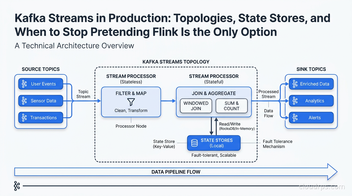
Kafka Streams consumes from Kafka topics, processes records, maintains local state, and writes results back to Kafka topics. The processing graph is called a topology. Each node in the topology is either a source (a topic you read from), a processor (business logic), or a sink (a topic you write to). State stores live alongside processors and are backed by changelog topics in Kafka itself, which is how Kafka Streams achieves fault tolerance without an external state service.

This is fundamentally different from Apache Flink, which runs as a cluster where you submit jobs. Flink has its own resource manager, its own checkpoint coordination, its own task scheduling. That infrastructure is real overhead, and it is worth carrying when you need Flink’s capabilities. When you do not, it is an unnecessary burden.

The Topology Model

Kafka Streams exposes two APIs for building topologies.

The high-level DSL gives you a fluent, declarative interface: KStream, KTable, GlobalKTable, and a chain of operations like filter, map, groupBy, aggregate, join. It is expressive and readable and handles most use cases.

StreamsBuilder builder = new StreamsBuilder();

KStream<String, Order> orders = builder.stream("orders");
KTable<String, CustomerProfile> customers = builder.table("customers");

KStream<String, EnrichedOrder> enriched = orders
    .join(customers,
          (order, customer) -> new EnrichedOrder(order, customer),
          Joined.with(Serdes.String(), orderSerde, customerSerde));

enriched.to("enriched-orders");

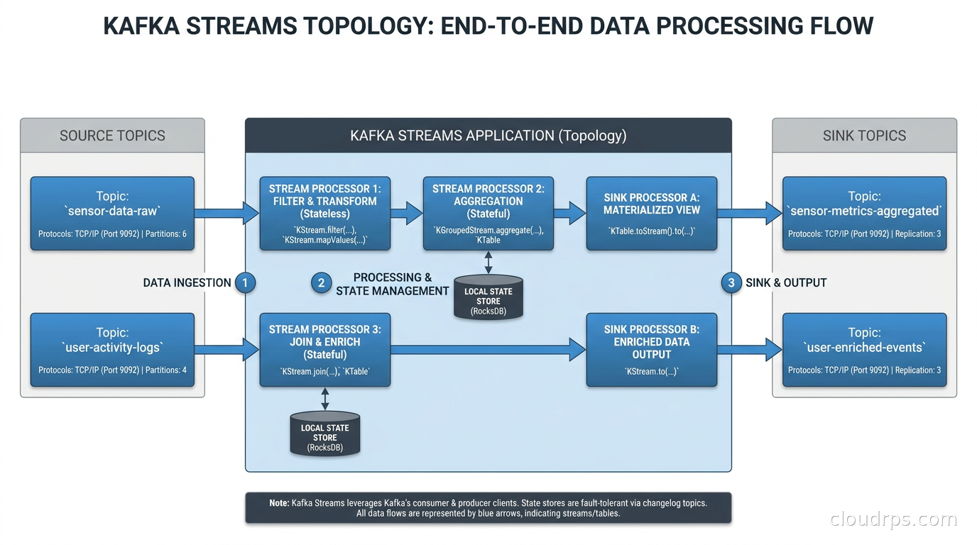
The low-level Processor API gives you explicit control over when to forward records downstream, how to schedule punctuation (time-driven callbacks), and how to interact with state stores directly. You implement the Processor interface and wire processors together explicitly. It is verbose but sometimes necessary, particularly for complex windowing logic, record-level timing control, or when the DSL abstractions leak in ways that cause behavior you cannot explain.

My recommendation: start with the DSL. If you hit a wall, migrate to the Processor API for the specific processor that needs it. The two APIs interoperate, so you can mix them within a single topology.

One operational detail that burned my team early: Kafka Streams creates internal topics for repartitioning when you use stateful operations. If you call groupBy on a key different from the partition key, Kafka Streams repartitions the data through an intermediate topic before aggregating. These repartition topics are created automatically, but they consume broker storage and add latency. Design your data models to partition on the key you will aggregate on, and you avoid the repartition hop.

State Stores and RocksDB

The differentiating feature of Kafka Streams is stateful processing with local state stores. By default, Kafka Streams uses RocksDB as the backing store for persistent state: a key-value store that runs embedded in your JVM process and stores data on local disk.

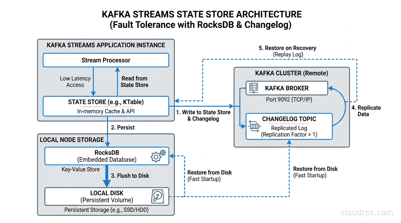
RocksDB is excellent for this use case. It handles high write throughput, supports range scans, and keeps its memory footprint manageable through configurable block cache and write buffer settings. The state stores Kafka Streams builds on top of RocksDB (through the RocksDBConfigSetter interface) are further tuned by default for stream processing access patterns.

For smaller state, you can use in-memory stores. These are faster but are lost on restart: the application replays the changelog topic to rebuild them. The rebuild time can be significant if you have accumulated days or weeks of state. I have seen teams make the mistake of using in-memory stores for tables they assumed were small, then discover that “small” at the start of a service lifecycle grows to hours of replay time by the time the service is two years old. Use persistent RocksDB stores by default. Use in-memory stores when you can bound the state size and you understand the restart behavior.

Each state store has a corresponding changelog topic in Kafka. Every write to the state store produces a record to the changelog topic. When a Kafka Streams instance fails or a partition is reassigned during scaling, the new instance replays the changelog to restore state. This is Kafka Streams’ fault tolerance mechanism, and it works well. The catch is that changelog replay can be slow for large state. Kafka Streams 2.6 added a standby replica feature: you configure additional instances that maintain warm copies of state, dramatically reducing recovery time. Configure num.standby.replicas for latency-sensitive applications. The tradeoff is higher broker storage consumption since standby replicas maintain their own changelog copies.

One operational concern worth repeating: on Kubernetes, state stores live on ephemeral pod storage by default. When a pod is rescheduled, it loses its local RocksDB state and replays from the changelog. For large state, this can take minutes and means your consumers sit idle during replay. Use a persistent volume (PVC) for the Kafka Streams state directory and configure sticky pod scheduling so that rescheduled pods land on the same node as their previous PV, or at minimum ensure the PV can be remounted quickly. This is the same class of problem that affects any stateful workload on Kubernetes.

Interactive Queries: The Feature Nobody Warns You About

Interactive queries let you expose your Kafka Streams state stores over an HTTP (or any RPC) interface so external callers can query the materialized state without hitting a database or Kafka itself. It sounds wonderful. In practice, it has constraints you must understand before you design your system around it.

The core issue: each Kafka Streams instance holds only the partitions assigned to it. If your topic has 12 partitions and you have three application instances, each instance holds state for four partitions. A query for a specific key arrives at whatever instance your load balancer routes it to. If that instance holds the partition for that key, the query succeeds. If not, the application must forward the request to the correct instance.

Kafka Streams exposes queryMetadataForKey() to find which instance holds a given key’s partition. Your application is responsible for implementing the forwarding layer: query the metadata, determine whether the key is local, and proxy to the correct instance if it is not. This is real application code you have to write and maintain.

// Your application must implement the routing layer
KeyQueryMetadata metadata = streams.queryMetadataForKey(
    "my-store",
    key,
    Serdes.String().serializer()
);

if (metadata.activeHost().equals(thisInstance)) {
    // local read
    ReadOnlyKeyValueStore<String, MyValue> store =
        streams.store(StoreQueryParameters.fromNameAndType(
            "my-store",
            QueryableStoreTypes.keyValueStore()
        ));
    return store.get(key);
} else {
    // forward to metadata.activeHost()
    return forwardToInstance(metadata.activeHost(), key);
}

If you want something more managed, the Interactive Queries API in newer Kafka Streams versions added pluggable QueryExecutors and improved the metadata API. Kafka 4.4.0 (October 2026) added KIP-1340 which improves GlobalKTable join handling, but the core routing-is-your-problem constraint remains. For most applications that need interactive query, I recommend building a thin microservice that handles the routing explicitly and exposes a clean API surface to callers. Treat the Kafka Streams instances as the state tier, not the query tier.

If interactive queries are central to your use case and the routing complexity is unappealing, look at streaming databases like RisingWave or Materialize which handle distributed query routing natively.

Exactly-Once Semantics in Practice

Kafka Streams supports exactly-once semantics through Kafka’s transactional API. Configure processing.guarantee=exactly_once_v2 (the improved implementation introduced in Kafka 2.6) and Kafka Streams will wrap reads, state store writes, and output topic writes in a single atomic transaction. If processing fails and restarts, the transaction is rolled back and the record is reprocessed without producing duplicate output.

There are real costs. EOS adds producer transaction overhead, requires additional broker interactions for transaction coordination, and reduces throughput compared to at-least-once delivery. The overhead varies by use case and topology complexity. At-least-once is the right default for idempotent operations (transformations, enrichments where duplicate writes are harmless). EOS matters when you are updating aggregates or counters where duplicate processing corrupts your result.

As of Kafka 4.0, the minimum supported broker version for Kafka Streams clients is 2.1. If you are running very old brokers, that is a constraint to verify before upgrading the library. The 4.0 release also dropped support for Java 8 and 11; you need Java 11 as a minimum for the client, and Java 17 for brokers and tooling. Plan your Java runtime upgrades if you are on older JVMs.

For schema management, Kafka Streams works naturally with Avro and Protobuf through the Confluent Schema Registry serializers. Register your schemas and use SpecificAvroSerde or KafkaProtobufSerde for type-safe deserialization. Schema evolution is straightforward when you follow backward-compatible changes. Breaking changes in your message schema will break your topology until you deploy updated consumers, so schema governance matters especially for state stores that persist across application versions.

Windowed Aggregations

Windowed aggregations are where Kafka Streams earns its keep for time-series analysis. The DSL supports tumbling windows, hopping windows, sliding windows, and session windows out of the box.

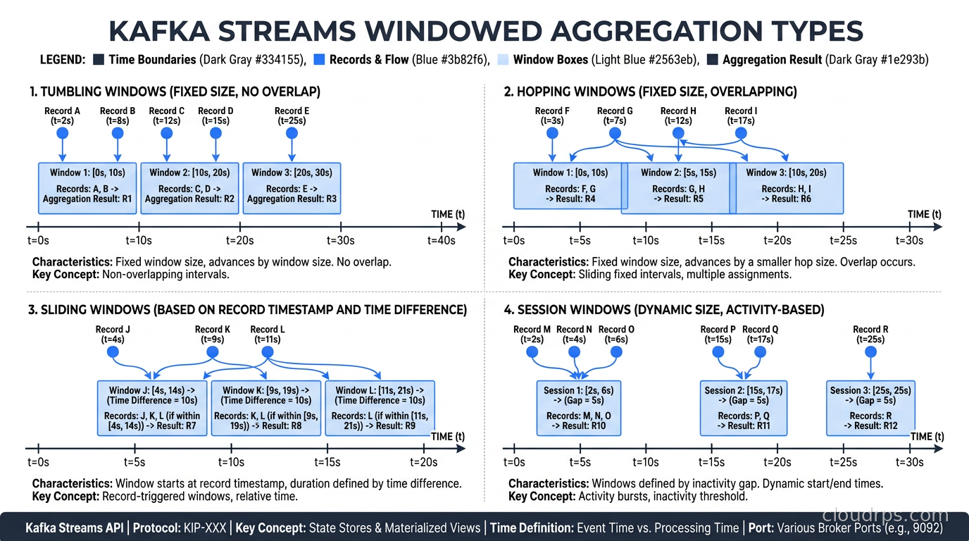
The critical operational concern for windowing is event-time versus processing-time. By default, Kafka Streams can operate on record timestamps (event time extracted from the Kafka record metadata), which is the right choice for most analytics use cases. However, late-arriving events are a production reality. Configure grace() on your window definitions to hold windows open for a configurable grace period after the window close time. Without a grace period, late events are dropped silently, and your aggregation results are quietly wrong.

Window state stores grow until the window retention period passes. Configure retention() on your materialized view to control how long historical window results are retained. For large windows or high-cardinality keys, window state can become significant. I have seen window state grow to hundreds of gigabytes on topics with high-cardinality user IDs and long retention settings. Monitor your state store sizes via Kafka Streams metrics and tune your window retention to what your use case actually requires.

Testing Your Topology

This is an area where Kafka Streams genuinely shines over Flink: testing is excellent. The TopologyTestDriver runs your complete topology in-process without a running Kafka cluster. You pipe records in, run the topology, and assert on output records and state store contents. Tests run in milliseconds.

@Test
void testOrderEnrichment() {
    TopologyTestDriver testDriver = new TopologyTestDriver(topology, props);

    TestInputTopic<String, Order> orderTopic = testDriver.createInputTopic(
        "orders", Serdes.String().serializer(), orderSerde.serializer()
    );
    TestOutputTopic<String, EnrichedOrder> outputTopic = testDriver.createOutputTopic(
        "enriched-orders", Serdes.String().deserializer(), enrichedSerde.deserializer()
    );

    orderTopic.pipeInput("user-1", new Order("item-A", 2));
    EnrichedOrder result = outputTopic.readValue();
    assertThat(result.customerName()).isEqualTo("Alice");
}

You can also advance event time explicitly in tests to verify windowing behavior. This makes testing complex windowing logic deterministic and fast, which is rare in stream processing. Build comprehensive topology tests before you deploy to production. The investment pays back quickly in production incidents caught in CI.

Deployment and Operational Considerations

Kafka Streams applications are plain Java applications. You containerize them and deploy them however you deploy your other services. Scaling is as simple as adding more instances: Kafka partitions are distributed across instances automatically through the Kafka Streams group management protocol.

For Kubernetes deployments, the main considerations are:

State store persistence. As I mentioned earlier, use PVCs for the state directory. Configure state.dir in your Streams config to point to the mounted volume path. Use StatefulSet rather than Deployment so each pod gets a stable identity and can be matched to its previous PV.

Scaling. When you add instances, Kafka Streams triggers a rebalance. During rebalance, processing pauses. Plan your scaling events accordingly. Configure num.standby.replicas to reduce the state rebuild time when partitions move to new instances. The KIP-848 rebalancing protocol (now the default in Kafka 4.0) applies to Kafka Streams groups as well and reduces pause duration.

JVM tuning. Kafka Streams applications under load benefit from explicit GC tuning. G1GC is the typical choice; ZGC is worth exploring if you have latency-sensitive workloads and can accept slightly higher throughput overhead. Configure heap size with enough headroom for the RocksDB off-heap block cache (which lives in native memory, outside the Java heap) and the in-flight processing buffers.

Kafka Streams metrics. The library emits a comprehensive set of JMX metrics: processing rate, state store read/write rate, standby restore lag, commit latency, and more. Expose these via JMX to Prometheus (using the JMX exporter) and build dashboards for them. The most important metrics to alert on are task-level restore lag (indicates slow standby rebuild), process rate drops (indicates upstream lag or processing errors), and commit failures.

The Honest Comparison with Flink and ksqlDB

Pick Kafka Streams when: your workload is Kafka-to-Kafka, your team is comfortable in Java, you want to avoid a separate cluster, your state volume is manageable (under a few hundred GB per partition), and your topology fits in the DSL model without requiring custom resource management.

Pick Apache Flink when: you have multiple input sources beyond Kafka, you need very large state (terabytes), your topology has complex operator graphs that benefit from Flink’s task-level scheduling, you need Flink SQL for analyst-accessible queries, or you need true multi-tenancy with resource isolation between jobs.

Pick a streaming database like RisingWave when: you need SQL-first development, you want managed incremental view maintenance, or your team is not comfortable with Java stream processing code.

Avoid ksqlDB for new projects. ksqlDB is built on Kafka Streams under the hood and was Confluent’s SQL interface for it. Confluent has strategically shifted investment toward Flink SQL as their preferred query layer. ksqlDB continues to work and has a user community, but the development velocity has moved elsewhere. If you want SQL-first stream processing today, Flink SQL is the more future-proof investment.

The Kafka Connect ecosystem complements Kafka Streams well. Use Connect to ingest data from external systems into Kafka topics and to export processed results to downstream systems. Kafka Streams sits in the middle, handling the stateful transformation logic. This three-tier pattern (ingest via Connect, process via Streams, export via Connect) is a clean architecture for many data engineering pipelines and avoids the need for direct database connectors in your Streams application.

For enforcing the shape of data flowing through your topologies, data contracts and schema governance matter. When your Streams application enriches an order with customer data and produces to an output topic, consumers of that output topic depend on a stable schema. Treat your Kafka Streams output topics as data products with defined schemas and compatibility guarantees.

Common Production Mistakes

I will close with the mistakes I see most often.

Unbounded state growth. Developers build a KTable that materializes all events without thinking about retention. The table grows indefinitely. Configure retention on Materialized views explicitly.

Repartition topic proliferation. Every groupBy on a non-partition key creates a repartition topic. These add latency and storage. Design your Kafka topic keys to match your aggregation keys.

Ignoring deserialization exceptions. Kafka Streams’ default behavior on a deserialization error is to log and continue. That means silently dropping records that do not match your schema. Configure a DeserializationExceptionHandler to either send malformed records to a dead-letter topic or halt and alert. Silent record drops in a production pipeline are insidious.

Testing against a live Kafka cluster. Unit tests that spin up a local Kafka are slow and flaky. Use TopologyTestDriver for unit tests and integration test environments for end-to-end validation.

Not configuring num.standby.replicas. The default is zero. After a pod restart with large state, you are waiting for changelog replay. Set this to one for latency-sensitive services.

Kafka Streams is not glamorous. It does not have a conference circuit, flashy vendor backing, or a dedicated operations team at most companies. What it has is two decades of battle-hardening in production Kafka environments, a testing story that is genuinely excellent, and an operational simplicity that most of its competitors cannot match for the right class of workload. When the problem fits, it fits better than the alternatives. Know when the problem fits.