LLM Inference Infrastructure: A Practical Guide to Serving AI Models at Scale

The first time I deployed an LLM to production, I thought I had it figured out. We had a fine-tuned 13B parameter model, a couple of A100 GPUs, and a Flask wrapper that accepted HTTP requests and returned completions. Ship it, right?

Within 48 hours, we had a P99 latency of 14 seconds, GPU memory errors crashing the service every few hours, and a cloud bill that made our VP of Engineering send me a Slack message consisting entirely of question marks. The model worked great on my laptop with one request at a time. Serving it to 200 concurrent users was an entirely different animal.

That experience taught me something that every cloud architect eventually learns the hard way: inference infrastructure is its own discipline. It borrows concepts from traditional web serving, but the constraints are fundamentally different. You are not just routing requests and returning database rows. You are managing GPU memory like a precious resource, optimizing for token throughput instead of requests per second, and making tradeoffs between latency and cost that do not exist in CPU-bound workloads.

I have spent the last three years building and rebuilding LLM inference stacks across multiple organizations. Here is what I wish someone had told me at the start.

Why Inference Is Not Training (And Why That Matters)

This distinction trips up a lot of teams. Training and inference both use GPUs, both involve large models, and both cost serious money. But the infrastructure requirements are almost opposite in important ways.

Training is throughput-oriented. You want to push as many tokens through the model as fast as possible, and you do not care about individual request latency because there are no individual requests. Training workloads are predictable, long-running, and batch-oriented. You can schedule them overnight, use spot instances aggressively, and tolerate failures because checkpointing lets you resume.

Inference is latency-sensitive and unpredictable. Real users are waiting for responses. Traffic patterns are bursty. You need to handle variable-length inputs and outputs. And here is the part that really makes inference tricky: you are doing autoregressive generation, meaning every token depends on the previous one. You cannot parallelize the generation of a single response the way you can parallelize a training batch.

This fundamental difference drives almost every infrastructure decision you will make. If you are coming from a training background and trying to apply the same patterns to inference, you will over-provision GPUs, under-optimize for latency, and spend far more money than necessary. The scalability and elasticity tradeoffs that matter for traditional web applications take on a whole new dimension when each “server” costs $2-8 per hour in GPU compute.

GPU Selection: Matching Hardware to Workload

Let me save you weeks of benchmarking and vendor calls. GPU selection for inference comes down to three factors: model size, latency requirements, and budget. Here is how I think about the major options.

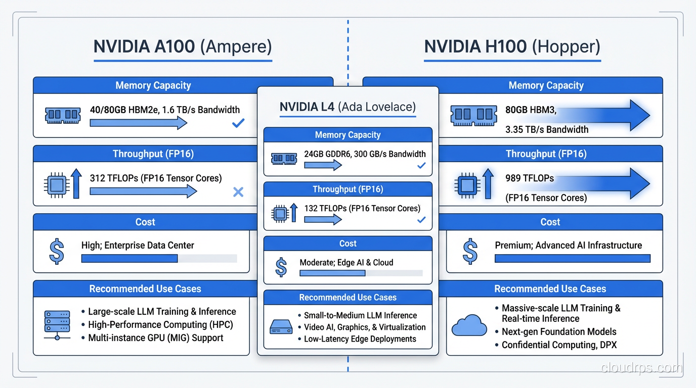
NVIDIA A100 (40GB and 80GB)

The A100 is the workhorse. It is not the newest or fastest, but it is available, well-supported by every framework, and the price-to-performance ratio is hard to beat for most inference workloads. The 80GB variant can fit a 70B parameter model with INT8 quantization, which covers the vast majority of production use cases.

I default to A100s unless I have a specific reason not to. They are the Honda Civic of inference GPUs: not flashy, but reliable, well-understood, and cost-effective.

NVIDIA H100

The H100 is significantly faster than the A100 for inference, particularly for large batch sizes and long sequence lengths. The Transformer Engine and improved memory bandwidth make a real difference. But they cost roughly 2-3x more per hour, and availability can be tight.

I recommend H100s when you have strict latency requirements on large models (70B+), when you are doing high-throughput batch inference and can saturate the GPU, or when your workload benefits from FP8 compute. If you are serving a 7B model to moderate traffic, H100s are overkill. You are paying for horsepower you will never use.

NVIDIA L4

The L4 is the sleeper pick. It is a Turing-based inference GPU that draws only 72 watts, fits in standard server slots, and costs a fraction of what A100s cost. For smaller models (up to 13B with quantization), the L4 delivers surprisingly good inference performance.

I have deployed L4-based inference for internal tools, development environments, and low-traffic production workloads. The cost savings are substantial. Just do not try to run a 70B model on them.

The Real-World Decision

In practice, most teams end up with a mix. L4s for smaller models and dev/staging environments. A100s for production workloads with moderate traffic. H100s reserved for the highest-traffic, most latency-sensitive endpoints. This tiered approach maps well to how different compute tiers work in cloud environments generally.

Model Serving Frameworks: The Engine Room

Picking the right serving framework matters more than most teams realize. The difference between a naive PyTorch inference loop and a purpose-built serving framework can be 5-10x in throughput. I have evaluated all the major options in production settings.

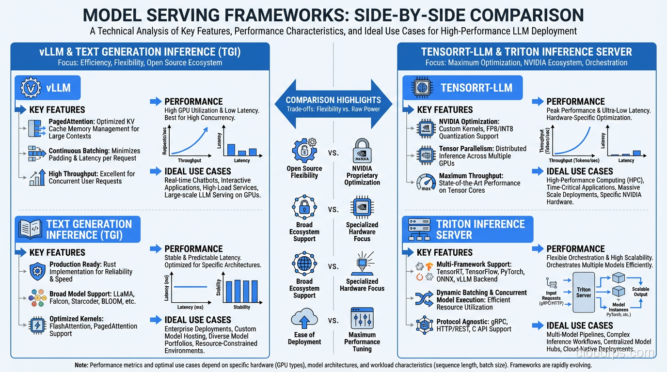
vLLM

vLLM is my default recommendation for most teams. Its killer feature is PagedAttention, which manages GPU memory for the KV cache the way an operating system manages virtual memory. Instead of pre-allocating fixed memory blocks for each request, vLLM dynamically allocates memory pages as tokens are generated. This dramatically improves GPU memory utilization and lets you serve more concurrent requests on the same hardware.

In my testing, vLLM consistently achieves 2-4x the throughput of a vanilla HuggingFace Transformers setup. The API is clean, it supports continuous batching out of the box, and the community is excellent. If you are starting fresh, start here.

TensorRT-LLM

NVIDIA’s TensorRT-LLM squeezes maximum performance out of NVIDIA hardware through aggressive kernel fusion and optimization. It can outperform vLLM on raw throughput, especially on H100s. The catch is that it requires a compilation step where you convert your model to a TensorRT engine, and this compilation is hardware-specific. An engine built for A100 will not run on H100.

I use TensorRT-LLM when I have a stable model that is not changing frequently and I need every last bit of performance. The compilation overhead and reduced flexibility are worth it when you are serving millions of requests per day on a model you update monthly.

Triton Inference Server

Triton is less a serving framework and more an inference orchestration platform. It supports multiple backends (including TensorRT-LLM, ONNX, and PyTorch), handles model versioning, and provides ensemble pipelines where you can chain preprocessing, inference, and postprocessing steps.

I reach for Triton when I have complex inference pipelines (for example, a tokenizer step, then the LLM, then a classifier on the output) or when I need to serve multiple model types from the same infrastructure. It adds operational complexity, but the flexibility is worth it for sophisticated deployments.

Text Generation Inference (TGI)

HuggingFace’s TGI is a solid option, particularly if your workflow is already HuggingFace-centric. It supports continuous batching, quantization, and most popular model architectures. Performance is competitive with vLLM for many workloads, though vLLM generally edges it out on throughput for larger models.

TGI shines when you want a well-documented, Docker-friendly deployment that integrates seamlessly with the HuggingFace ecosystem. For teams already using HuggingFace for model management, TGI reduces the operational surface area.

Batching Strategies: Where the Real Throughput Lives

If you take one thing from this article, let it be this: batching strategy is the single biggest lever you have for inference throughput. A well-tuned batching configuration can improve throughput 3-5x over naive one-request-at-a-time serving.

Static Batching (Do Not Do This)

Static batching collects a fixed number of requests, pads them to the same length, processes them together, and returns results when the entire batch completes. This is how most people start, and it is terrible for LLM inference. The problem is that requests have wildly different input and output lengths. When you pad a 10-token input to match a 500-token input in the same batch, you waste enormous amounts of compute. And every request in the batch waits for the longest response to finish generating.

Continuous Batching

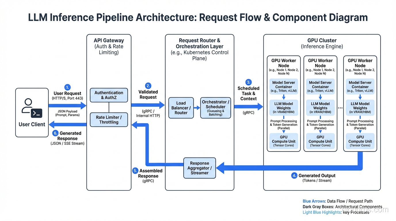
Continuous batching (also called iteration-level batching) is the correct approach. Instead of waiting for an entire batch to complete, the system processes one token generation step at a time across all active requests. When a request finishes generating, its slot immediately opens for a new request without waiting for the rest of the batch.

This is analogous to how modern web servers handle connections versus old-school thread-per-request models. The GPU stays busy generating tokens rather than sitting idle while shorter requests wait for longer ones. Both vLLM and TGI implement continuous batching, and it is the primary reason they achieve such high throughput.

Dynamic Batching with Priority

In production, you often have requests with different priority levels. A real-time chatbot response needs sub-second time-to-first-token. A batch summarization job can tolerate seconds of queue time. Dynamic batching with priority queues lets you ensure that high-priority requests get GPU cycles immediately while lower-priority work fills in the gaps.

I implement this with a request router that sits in front of the inference server, classifying requests by priority and managing queue depths. This is where your load balancing strategy becomes critical, because you need to route requests to GPU instances that have capacity without introducing unacceptable queuing delays.

Quantization and Optimization: Trading Precision for Speed

Quantization reduces model weights from their training precision (usually FP16 or BF16) to lower precision formats, shrinking the model’s memory footprint and often improving inference speed. The tradeoff is a small reduction in output quality, though modern quantization techniques have made this surprisingly minimal.

INT8 Quantization

INT8 is the safest starting point. It halves the memory footprint compared to FP16, which means a model that required two GPUs can fit on one. For most applications, the quality degradation is negligible. I have deployed INT8 quantized models where the product team could not distinguish the outputs from the full-precision version in blind evaluations.

Use INT8 when you want a straightforward memory reduction with minimal risk. Both bitsandbytes and GPTQ support INT8, and most serving frameworks handle it natively.

GPTQ (4-bit)

GPTQ is a post-training quantization method that compresses models to 4-bit precision. The memory savings are dramatic: a 70B parameter model that normally requires 140GB in FP16 can fit in roughly 35GB with GPTQ, meaning it runs on a single A100-80GB.

The quality impact varies by model and task. For creative text generation, I have seen noticeable degradation. For classification, extraction, and structured output tasks, GPTQ models perform nearly identically to their full-precision counterparts. Always benchmark on your specific use case before committing.

AWQ (Activation-Aware Weight Quantization)

AWQ is a newer approach that selectively protects the most important weights during quantization based on activation patterns. In my experience, AWQ consistently produces better output quality than GPTQ at the same bit-width. The inference speed is comparable, and framework support has matured rapidly.

I have been defaulting to AWQ over GPTQ for new deployments. The quality advantage is small but consistent, and there is no meaningful performance penalty.

When to Quantize (and When Not To)

Quantize when you are memory-constrained (model does not fit on your target GPU at full precision), when you need to reduce cost by using fewer or smaller GPUs, or when latency matters more than output quality at the margins.

Do not quantize when you are serving a small model that fits comfortably in GPU memory at full precision, when output quality is absolutely paramount and you have the budget for full-precision serving, or when you are still iterating on the model and need to isolate quality issues from quantization artifacts.

Cost Optimization: Making the CFO Happy

GPU inference is expensive. A single A100 instance on AWS costs roughly $3-4 per hour. At scale, inference costs can dwarf your training budget. Here are the strategies I have found most effective for controlling costs without sacrificing reliability.

Spot Instances for Inference (Yes, Really)

Most architects shy away from spot instances for serving workloads because of the interruption risk. But with the right architecture, spot instances work well for inference. The key is treating your inference fleet as a pool with graceful degradation.

Run a small on-demand base capacity that handles your minimum traffic. Layer spot instances on top for burst capacity. Use a request queue so that when a spot instance gets reclaimed, in-flight requests can be retried on surviving instances. The savings are 60-70% compared to on-demand pricing.

This requires proper high availability design, but the cost reduction is significant enough to justify the engineering investment. I have run inference fleets at 80% spot composition with P99 availability above 99.9%.

Autoscaling for Inference

Traditional CPU-based autoscaling metrics do not work for GPU workloads. Scaling on CPU utilization is meaningless when the bottleneck is GPU compute. Instead, scale on these metrics:

GPU utilization is the most obvious metric, but it can be misleading. A GPU at 90% utilization might be handling the load fine, or it might be backed up with a growing queue. Always pair GPU utilization with queue depth.

Request queue depth is the most actionable scaling signal. When your request queue grows beyond a threshold (I typically use 10-20 pending requests per GPU), scale up. When it drops to zero consistently, scale down.

Time-to-first-token (TTFT) is the metric your users actually feel. If TTFT starts exceeding your SLA (usually 200-500ms for interactive applications), that is an unambiguous signal to add capacity.

Setting up these custom metrics requires solid monitoring and logging infrastructure, which I consider non-negotiable for any production inference deployment.

Multi-Model Serving

If you are serving multiple models, consolidating them onto shared GPU infrastructure can dramatically reduce costs. Instead of dedicating GPU instances to each model, use a framework like Triton or vLLM’s multi-model support to serve several models from the same GPU pool.

The trick is memory management. You need to ensure that the combined memory footprint of all loaded models fits within GPU memory, or implement intelligent model swapping that loads and unloads models based on demand. This gets complex, but for organizations serving 5-10 different models, the cost savings justify the complexity.

Right-Sizing Requests

One optimization that is easy to overlook: controlling input and output token lengths. Every unnecessary token in the prompt costs compute. Every extra token in the response costs latency and money.

I have seen teams cut inference costs by 30-40% simply by optimizing their prompts to be more concise, setting appropriate max_tokens limits, and implementing response length controls. It is the least glamorous optimization, but often the most impactful.

Monitoring and Observability: Knowing What Is Actually Happening

Inference workloads require monitoring that goes beyond standard application metrics. Here are the signals I track and alert on.

Latency Metrics

Time-to-first-token (TTFT) measures how long a user waits before they see the first token of a response. For streaming applications, this is the most important user-facing metric. I target P50 under 200ms and P99 under 500ms for interactive use cases.

Inter-token latency (ITL) measures the gap between consecutive tokens during generation. Spikes in ITL indicate GPU contention or memory pressure. Consistent ITL means your serving infrastructure is healthy.

End-to-end latency is important for non-streaming applications where users wait for the complete response. This is heavily influenced by output length, so track it as a distribution, not just an average.

Throughput Metrics

Tokens per second per GPU is the core throughput metric. It tells you how efficiently you are using your hardware. Track this for both input tokens (prefill phase) and output tokens (decode phase) separately, because they stress the GPU differently.

Requests per second still matters, but it is less informative than tokens per second because request sizes vary enormously. A system handling 10 requests per second with 50-token outputs is doing very different work than one handling 10 requests per second with 2000-token outputs.

Resource Utilization

GPU memory utilization should be monitored continuously. Memory leaks in inference servers are more common than you would expect, and running out of GPU memory means OOM kills and dropped requests. I alert at 85% memory utilization and investigate at 90%.

GPU compute utilization shows how busy the GPU cores are. For a well-optimized inference workload, you want this in the 70-90% range. Below 50% means you are over-provisioned. Above 95% means you are likely queuing requests.

Understanding the relationship between latency and bandwidth takes on a specific meaning in GPU inference: memory bandwidth is often the bottleneck for autoregressive decoding, not raw compute. Monitoring memory bandwidth utilization can reveal optimization opportunities that compute metrics alone would miss.

Alerting Strategy

My standard alerting configuration for inference:

• Page (immediate response needed): TTFT P99 exceeds 2 seconds, GPU OOM events, request error rate above 1%.
• Warn (investigate within hours): GPU memory above 85%, request queue depth growing for 5+ minutes, TTFT P99 above 1 second.
• Info (review daily): Cost per 1000 tokens trending upward, throughput per GPU declining, model version drift across instances.

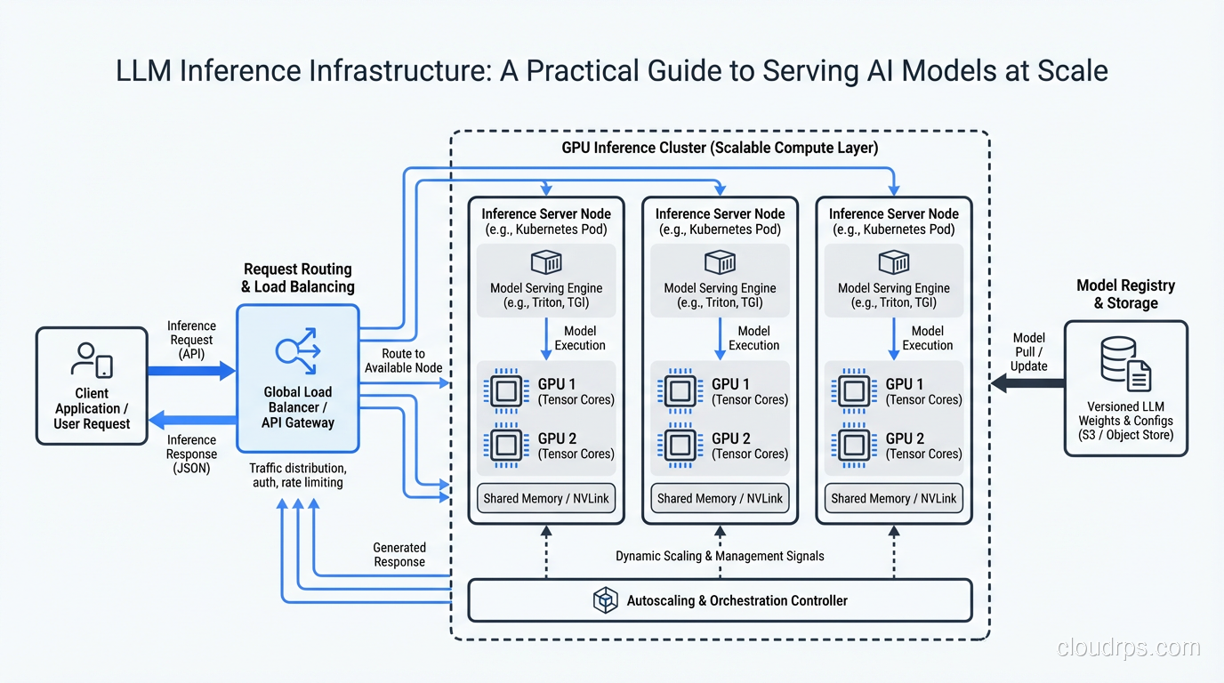
Putting It All Together: A Reference Architecture

For a team deploying their first production LLM inference stack, here is the architecture I recommend:

Start with vLLM on A100-80GB instances. Use AWQ quantization if your model benefits from it. Configure continuous batching with a max batch size of 32-64 (tune based on your sequence lengths). Put an async request router in front that handles priority queuing and retry logic. If your application uses RAG, you will also need a vector store for embeddings. For most teams, pgvector on PostgreSQL handles this without spinning up additional infrastructure; see the vector databases guide for when that is sufficient versus when a dedicated vector DB makes sense.

Use a standard load balancer with health checks that verify GPU availability, not just HTTP 200s. Your health check should confirm that the model is loaded and the GPU is responding. A server that returns 200 but has a crashed CUDA context is worse than a server that is down, because the load balancer keeps sending it traffic.

Implement autoscaling on queue depth and TTFT, with a minimum on-demand base and spot instances for burst capacity. Set up proper monitoring from day one, tracking the metrics I described above.

Plan for failure. GPU instances fail more often than CPU instances. CUDA errors, driver issues, and memory corruption are all part of the landscape. Design your system to gracefully handle instance failures, with automatic request retry and instance replacement. The principles of scaling web applications apply here, but the failure modes are different and the recovery time for spinning up a new GPU instance is longer.

This architecture will carry you from your first production deployment through tens of thousands of requests per hour. When you outgrow it, you will have enough operational experience to know exactly which components need to evolve and why.

The field is moving fast. New GPUs, new serving frameworks, and new optimization techniques emerge every few months. But the fundamentals I have covered here, understanding the unique constraints of inference workloads, matching hardware to requirements, optimizing batching and quantization, and monitoring the right signals, will remain relevant regardless of which specific tools you end up using. Build on solid foundations, measure everything, and iterate based on real production data rather than benchmarks and blog posts. Including this one.