PostgreSQL Indexing Strategies: B-tree, GIN, GiST, BRIN, and Knowing Which Index to Actually Use

There is a particular kind of 2am call I have gotten more times than I want to count. The pattern is always the same: a new feature ships in the afternoon, everything looks fine, and then by midnight the database is on its knees. Query latency has gone from 10ms to 12 seconds. The on-call engineer is staring at pg_stat_activity watching connections pile up. Revenue is bleeding.

The fix, almost every time, is a single CREATE INDEX statement that runs in a few minutes. Twenty years of building cloud infrastructure and I still see the same indexing mistakes repeat across teams. Not because engineers are careless, but because PostgreSQL’s indexing system is genuinely complex. You have six core index types, several specialized patterns, and a query planner that will silently ignore your index if it decides a sequential scan is cheaper. Getting it right requires understanding not just the data structures, but what the planner considers when it evaluates your query.

This is that guide.

Why Index Type Matters More Than You Think

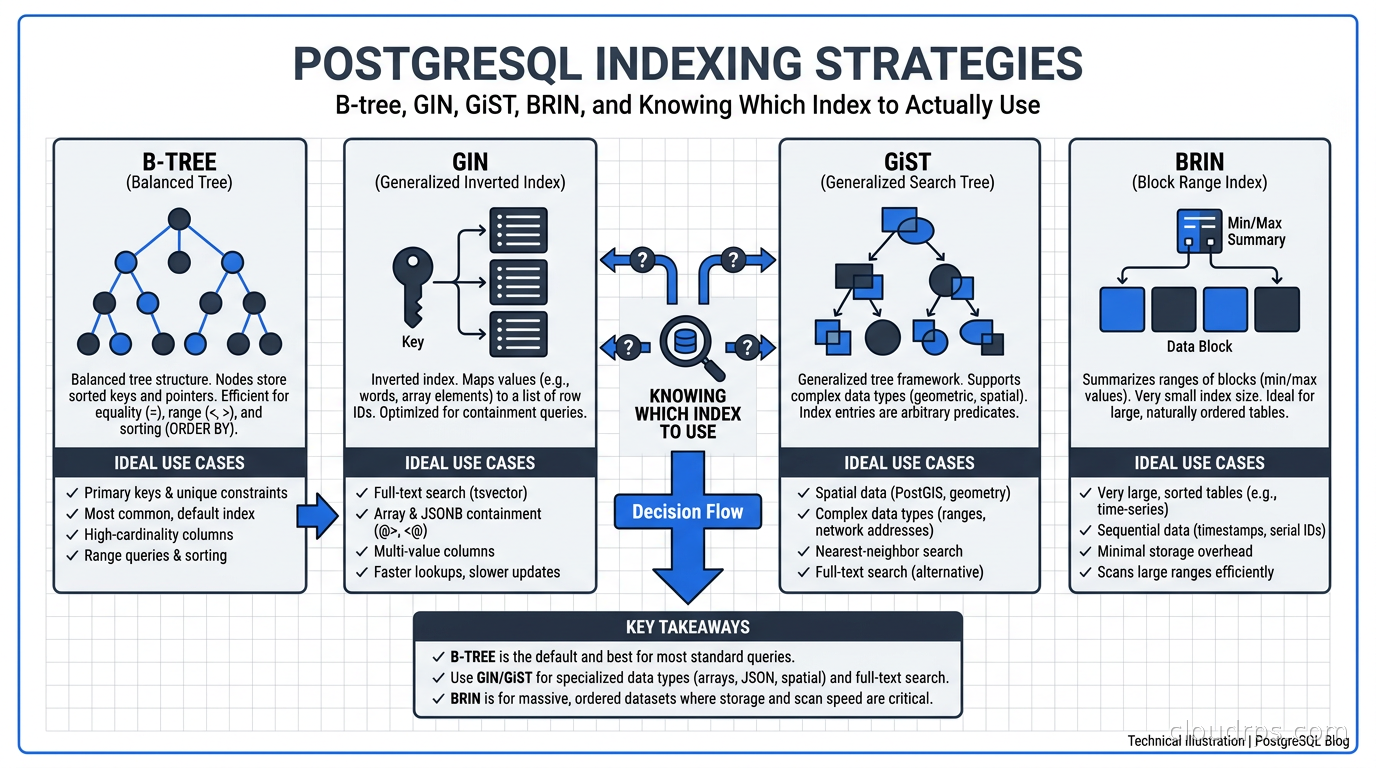
Most introductory material treats indexes as if there is basically one kind (B-tree) and everything else is exotic. That framing leads to real production pain. Using a B-tree index on a JSONB column will not help you query nested JSON keys. Putting a GIN index on a high-write table can slow inserts by 40%. A BRIN index on a randomly-ordered column returns nothing useful.

PostgreSQL’s index types map to specific data structures and query access patterns. Choosing the wrong one is nearly as bad as having no index at all.

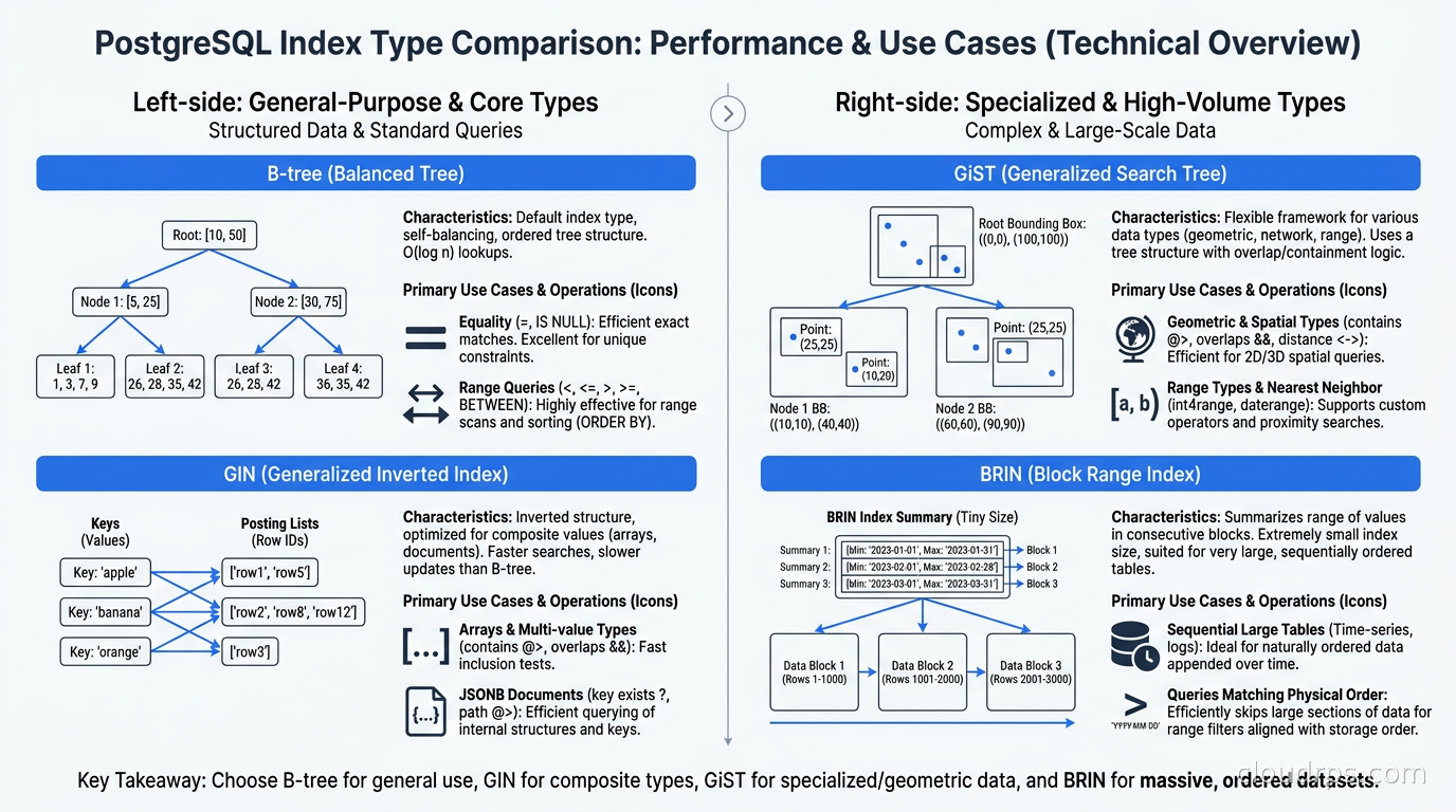
The decision process is not complicated once you internalize one principle: index types are designed around the operators your queries use. Equality and range queries use B-tree. Containment queries on composite values use GIN. Geometric proximity searches use GiST. Sequential-correlation tables use BRIN. Everything else follows from that.

B-tree: The Index You Use 95% of the Time

B-tree (Balanced Tree) is the default. Write CREATE INDEX with no type specified and you get a B-tree. It handles equality, range queries, and ordering: the bread and butter of most SQL workloads.

CREATE INDEX idx_orders_created_at ON orders(created_at);
CREATE INDEX idx_users_email ON users(email);

B-tree supports: =, <, <=, >, >=, BETWEEN, IN, IS NULL, IS NOT NULL, and LIKE with a left-anchored prefix (e.g., LIKE 'prefix%' works; LIKE '%suffix' does not).

The sorted tree structure is also why ORDER BY queries can skip a sort step entirely when a matching B-tree index exists. For pagination, this matters. A query with ORDER BY created_at DESC LIMIT 50 can walk the index leaf pages directly. The classic OFFSET pagination is still slow at large offsets (the planner has to skip through the index), but keyset pagination with a WHERE clause on the last-seen value becomes very fast with a proper B-tree index.

Where B-tree fails: Equality queries on very low-cardinality columns. A boolean column, or a status enum with three values spread roughly evenly across the table, will often be ignored by the planner. If an index lookup would return 30% of the table, PostgreSQL knows that random I/O through the index is slower than a single sequential scan. I have watched teams add an is_active index to a users table with 95% active rows and wonder why Postgres ignores it entirely. The planner is not broken. It is doing the math correctly. Use partial indexes for this case.

Hash: Fast Equality, Limited Value

Hash indexes trade flexibility for speed on exact-match lookups. They were historically unsafe (not WAL-logged before PostgreSQL 10) and are now reliable, but still rarely worth choosing over B-tree.

CREATE INDEX idx_sessions_token ON sessions USING HASH (token);

Hash indexes are smaller than B-trees for equality-only queries and marginally faster on very large tables. The major limitations: no range queries, no ordering, no multi-column support. Unless you have a billion-row table doing nothing but exact lookups on a single column, stick with B-tree. The planner can use a B-tree for equality just as well, and it keeps all the flexibility you will eventually need.

GIN: Arrays, JSONB, and Full-Text Search

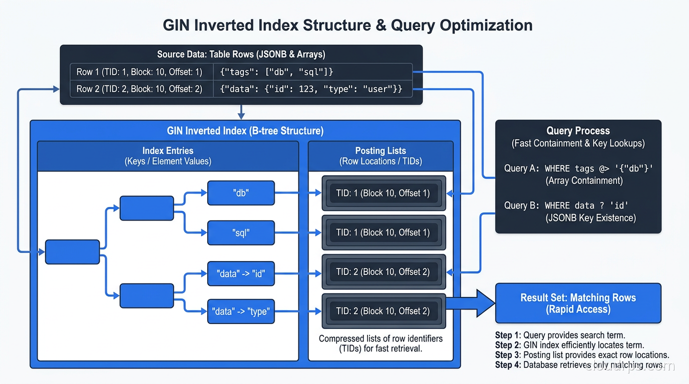
GIN (Generalized Inverted Index) is the right choice when a single column contains multiple indexable values. The canonical use cases are PostgreSQL arrays, JSONB columns, and full-text tsvector columns.

The inverted index structure maps each element value to the set of rows containing it. This is exactly how search engines index text, and it is why GIN is so effective for containment queries.

-- Array containment queries
CREATE INDEX idx_products_tags ON products USING GIN (tags);
SELECT * FROM products WHERE tags @> '{featured, sale}';

-- JSONB key/value queries with jsonb_path_ops (smaller, faster)
CREATE INDEX idx_events_payload ON events USING GIN (payload jsonb_path_ops);
SELECT * FROM events WHERE payload @> '{"type": "purchase"}';

-- JSONB with jsonb_ops (supports more operators)
CREATE INDEX idx_logs_data ON logs USING GIN (data jsonb_ops);
SELECT * FROM logs WHERE data ? 'error_code';

-- Full-text search
CREATE INDEX idx_articles_search ON articles USING GIN (search_vector);
SELECT * FROM articles WHERE search_vector @@ to_tsquery('postgresql & indexing');

The two JSONB operator classes have different tradeoffs. jsonb_path_ops is smaller and faster but only supports containment (@>). jsonb_ops is larger and supports key existence checks (?, ?|, ?&) as well. Choose based on which operators your queries actually use.

The write amplification trap: GIN indexes are expensive to maintain. Every INSERT or UPDATE touching an indexed column updates the inverted index structure, which may affect many posting list entries. PostgreSQL mitigates this with a pending list (GIN fast-update mode, enabled by default) that batches writes, but queries against a large pending list are slower until autovacuum or an explicit VACUUM flushes it.

On a write-heavy JSONB table at a previous client, I watched GIN maintenance consume 40% of database CPU during peak ingestion windows. The fix was disabling fast-update (fastupdate=off) and accepting slightly slower individual writes rather than the unpredictable flush storms. Know your write/read ratio before committing to GIN on high-throughput tables.

GiST: Geometric Data and Nearest-Neighbor Searches

GiST (Generalized Search Tree) is an extensible index framework PostgreSQL uses for geometric types (points, boxes, circles, polygons), range types (daterange, tsrange, int4range), and proximity queries.

-- Range type overlap queries
CREATE INDEX idx_bookings_period ON bookings USING GIST (period);
SELECT * FROM bookings WHERE period && '[2025-06-01,2025-06-07)';

-- Nearest-neighbor (KNN) search on points
CREATE INDEX idx_locations_coords ON locations USING GIST (coords);
SELECT * FROM locations ORDER BY coords <-> point(40.7128, -74.0060) LIMIT 10;

-- PostGIS geographic queries (requires PostGIS extension)
CREATE INDEX idx_stores_geom ON stores USING GIST (geom);
SELECT * FROM stores WHERE ST_DWithin(geom, ST_MakePoint(-74.006, 40.712)::geography, 1000);

GiST indexes are lossy by design: the index may return false positives, and PostgreSQL automatically re-checks each candidate row against the actual heap data. This adds a small amount of I/O, but for the geometric and range queries GiST handles, it is still orders of magnitude faster than sequential scans.

SP-GiST (Space-Partitioned GiST) is a variant for non-balanced partitioning structures: quad trees, k-d trees, radix trees. It works well for spatial data with natural clustering, IP address ranges, and phone numbers. Most applications reach for GiST first; SP-GiST becomes relevant only when you are deep into spatial queries with strong locality properties or prefix-structured data types.

If you are using PostGIS from the PostgreSQL extensions ecosystem, GiST is what powers all spatial indexing under the hood. Understanding GiST is prerequisite knowledge for tuning PostGIS query performance.

BRIN: The Right Index for Huge Sequential Tables

BRIN (Block Range Index) is the index nobody reaches for until they have a 500GB log table and realize a B-tree index on the timestamp column would be 50GB on its own.

BRIN works by storing min/max summaries for ranges of physical disk blocks. Instead of pointing to individual rows, it tells the planner “rows in blocks 0 through 128 have timestamps between 2025-01-01 and 2025-01-07.” Queries scan only the block ranges whose min/max overlaps with the search predicate.

-- Append-only event log with strongly correlated physical order
CREATE INDEX idx_events_ts ON events USING BRIN (occurred_at);

-- Customize pages per range (default 128, smaller = more precise but bigger index)
CREATE INDEX idx_events_ts ON events USING BRIN (occurred_at) WITH (pages_per_range = 32);

BRIN indexes are tiny. On a table with two billion rows, a BRIN index on a timestamp column might be under 1MB. A B-tree index on the same column would be tens of gigabytes. Beyond storage, BRIN is almost free to maintain: an insert to a new block simply updates the block range summary rather than inserting a key into a tree.

The catch is strong: BRIN only works when there is genuine physical correlation between the indexed column and the row’s location on disk. For a timestamp on an append-only table (rows written in order and never updated), that correlation is excellent. For a UUID column, or any column whose values are scattered randomly across the physical table, BRIN provides no benefit at all.

I have used BRIN on time-series event tables at the two-billion-row scale where a B-tree was impractical without horizontal partitioning. The BRIN index cut date-range query times from over an hour (sequential scan) to under two minutes. For append-mostly, time-ordered data, BRIN is one of the most underused tools in PostgreSQL.

Advanced Index Patterns

Partial Indexes

A partial index applies only to rows satisfying a WHERE clause. It is smaller, faster to build, cheaper to maintain, and the planner can use it for any query that implicitly or explicitly matches the filter.

-- Only index users who have not been deleted
CREATE INDEX idx_users_active_email ON users(email) WHERE deleted_at IS NULL;

-- Only index orders in an open state (a small fraction of all orders)
CREATE INDEX idx_orders_open_created ON orders(created_at) WHERE status = 'open';

-- Only index recent events (combined with a partitioning strategy)
CREATE INDEX idx_events_recent ON events(user_id) WHERE occurred_at > '2025-01-01';

Partial indexes are the answer to the low-cardinality problem. If 5% of users are active and 95% are deleted, a partial index on the 5% is 20 times smaller than a full index and the planner can use it reliably. I consider partial indexes the most underused optimization tool in the average PostgreSQL deployment. They should be your first instinct whenever you have a status or soft-delete column in query predicates.

Covering Indexes (INCLUDE Clause)

Introduced in PostgreSQL 11, covering indexes let you attach additional columns to an index without including them in the sort key. This enables index-only scans where PostgreSQL never touches the table heap at all.

-- User order lookup including fields commonly fetched together
CREATE INDEX idx_orders_user ON orders(user_id) INCLUDE (status, total_amount, created_at);

-- This query never touches the orders table heap:
SELECT status, total_amount, created_at FROM orders WHERE user_id = 12345 ORDER BY created_at;

Index-only scans are dramatically faster on large tables because they avoid the random I/O of heap fetches entirely. The tradeoff is index size: the INCLUDE columns are stored in every leaf node of the B-tree. Profile your read-versus-storage tradeoff before including many wide columns. A covering index that saves 50ms per query but doubles index storage costs might be worth it on a heavily-read table and wrong on a write-heavy one.

Expression Indexes

PostgreSQL can index the result of a function or expression, not just a raw column value. The query must use the same expression for the index to apply.

-- Case-insensitive email uniqueness and lookup
CREATE UNIQUE INDEX idx_users_lower_email ON users(lower(email));
SELECT * FROM users WHERE lower(email) = lower('User@Example.com');

-- Index an extracted JSONB field
CREATE INDEX idx_orders_customer_id ON orders((metadata->>'customer_id'));
SELECT * FROM orders WHERE metadata->>'customer_id' = 'cust_12345';

-- Index on extracted date portion
CREATE INDEX idx_events_date ON events(date_trunc('day', occurred_at));
SELECT * FROM events WHERE date_trunc('day', occurred_at) = '2025-05-15';

Expression indexes solve a common anti-pattern where developers apply functions to indexed columns in WHERE clauses, breaking index usability. The expression in the query must match the expression in the index exactly, including the same function arguments. lower(email) in the index works; email ILIKE 'foo%' uses it; email = 'Foo' does not.

Multicolumn Indexes and Column Order

Column order in composite indexes matters significantly and is the source of a large fraction of the indexing mistakes I review in production codebases.

-- (user_id, created_at): which queries does this support?
CREATE INDEX idx_orders_user_date ON orders(user_id, created_at);

-- Yes: leading column present
SELECT * FROM orders WHERE user_id = 42;

-- Yes: both columns used
SELECT * FROM orders WHERE user_id = 42 AND created_at > '2025-01-01';

-- No: only trailing column, no leading column
SELECT * FROM orders WHERE created_at > '2025-01-01';

The rule: a composite B-tree index can be used for queries that filter or sort on the leading N columns in order. Put the most-filtered or highest-selectivity column first. If you query on status AND user_id roughly equally, and user_id has much higher cardinality, lead with user_id. If a query needs only status, a separate single-column index on status (or a partial index) is better than the composite.

Index Maintenance and Bloat

PostgreSQL uses MVCC for concurrent reads and writes. Every UPDATE writes a new row version and marks the old one dead rather than overwriting in place. Over time, on write-heavy tables, dead row versions accumulate in both the table heap and in the index. Autovacuum reclaims this space, but on tables with very high update rates, it cannot always keep pace. The result is index bloat: the index grows physically larger than its live data.

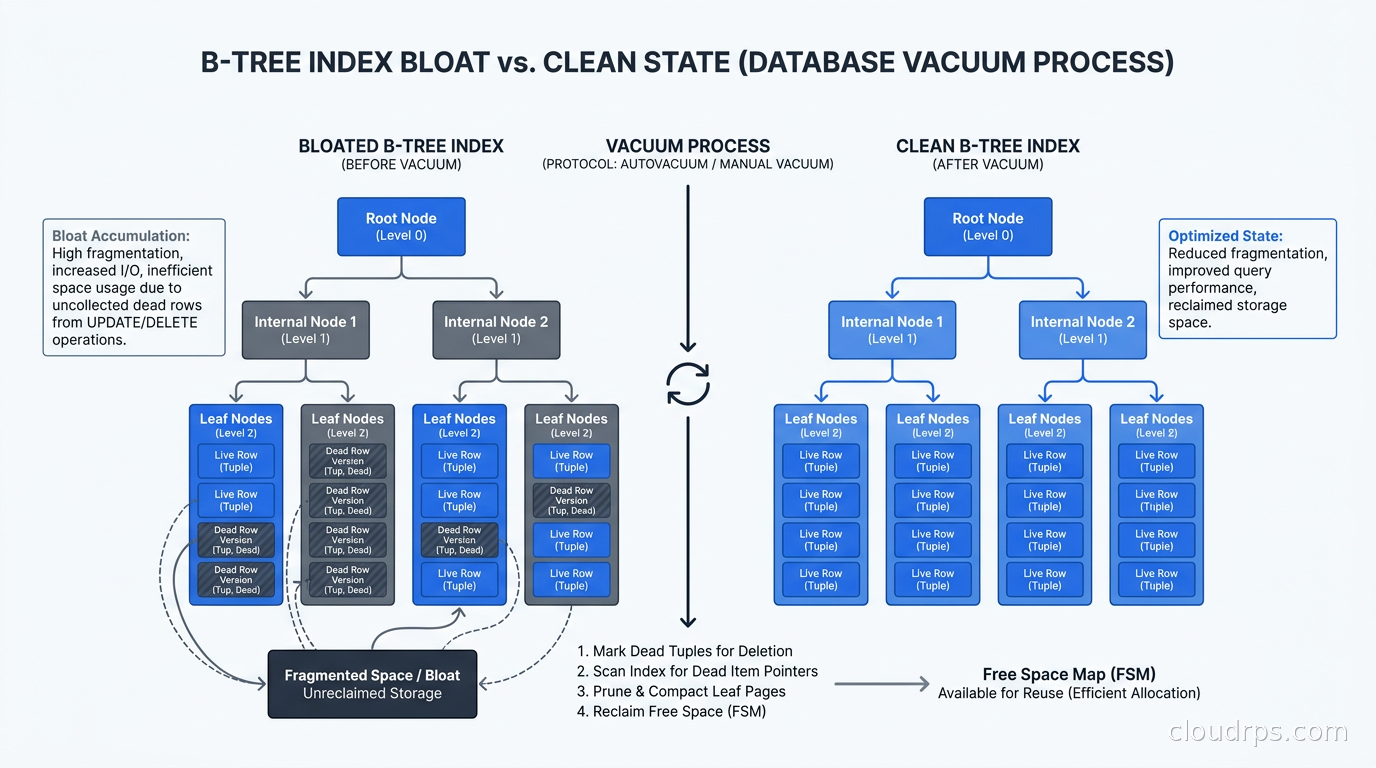
Bloated indexes cause measurable performance degradation: more I/O per query, higher buffer cache pressure, and slower maintenance passes. The pgstattuple extension can diagnose bloat:

CREATE EXTENSION pgstattuple;
SELECT index_size, leaf_fragmentation, avg_leaf_density
FROM pgstatindex('idx_orders_user_id');

When bloat is severe, REINDEX CONCURRENTLY rebuilds the index online without locking reads or writes:

REINDEX INDEX CONCURRENTLY idx_orders_user_id;

This is slow and resource-intensive but non-blocking. For tables under constant write pressure, I schedule monthly reindex jobs during maintenance windows. The zero-downtime database migration patterns I rely on include concurrent reindexing as a standard tool alongside pg_repack, which handles table bloat and index bloat in a single pass.

Creating indexes on live production tables also requires CONCURRENTLY to avoid table locks:

CREATE INDEX CONCURRENTLY idx_events_user_id ON events(user_id);

Without CONCURRENTLY, a CREATE INDEX holds an exclusive lock for the duration of the build. On a table with hundreds of millions of rows, that is minutes of lock time. I have watched a team lock their API for 22 minutes because they ran a CREATE INDEX without CONCURRENTLY on a 300-million-row table at noon on a Tuesday. Always use CONCURRENTLY in production. It takes longer and has more overhead, but the alternative is a hard outage.

Reading EXPLAIN ANALYZE

Indexes are only useful if the planner actually uses them. EXPLAIN ANALYZE is how you verify:

EXPLAIN (ANALYZE, BUFFERS, FORMAT TEXT)
SELECT * FROM orders WHERE user_id = 42 AND status = 'open';

The key plan nodes to understand:

Index Scan: The planner uses the index to find qualifying row pointers, then fetches each row from the heap. Good for selective queries returning a small fraction of rows.

Index Only Scan: The planner retrieves all needed data from the index without touching the heap. The best case, enabled by covering indexes or when all needed columns happen to be in the index. Watch the “Heap Fetches” line in the output; if it is non-zero, visibility map coverage may be incomplete and autovacuum needs to run.

Bitmap Index Scan + Bitmap Heap Scan: For queries returning a moderate number of rows, the planner collects all matching row pointers from the index into a bitmap first, then fetches heap pages in physical order. More efficient than repeated random heap I/O for mid-range selectivity.

Seq Scan: No index used. The planner scans the entire table. This is correct when the query would return a large fraction of rows, when the table is small, or when statistics are stale.

Stale statistics are a common culprit when indexes exist but get ignored. After bulk loads or significant data changes, table statistics may be outdated and the planner misjudges row counts. Running ANALYZE table_name refreshes statistics immediately. The relationship between write-ahead logging, autovacuum, and autoanalyze is worth understanding: autovacuum drives both the dead tuple cleanup and the statistics refresh that keeps the planner honest.

When NOT to Index

Adding indexes always has costs: storage, slower writes, autovacuum overhead, and bloat risk. Some columns should not be indexed at all.

Very low cardinality with uniform distribution. A gender column with three values evenly spread across the table will almost never get the planner to choose an index scan. Fetching 33% of the table via random I/O through an index is slower than a single sequential scan. Use partial indexes or accept the sequential scan.

Small tables. Under roughly 10,000 rows, sequential scans are fast enough that index overhead outweighs the benefit. The planner will typically choose the sequential scan anyway.

Write-heavy staging or ingestion tables. Raw event ingestion tables, log staging tables, ETL landing zones. Indexing every column collapses insert throughput. For these, I use no indexes or at most a BRIN on the timestamp, and move queryable data to a properly-indexed summary table or analytical store.

Non-sargable expressions without expression indexes. WHERE EXTRACT(YEAR FROM created_at) = 2025 cannot use an index on created_at. Either rewrite as WHERE created_at >= '2025-01-01' AND created_at < '2026-01-01', or create an expression index on EXTRACT(YEAR FROM created_at). The ACID properties and MVCC model also mean that highly concurrent updates to indexed columns have locking implications worth profiling before adding indexes to hot-path tables.

The Index Decision Framework

Before creating any index, work through this checklist:

1. Find the slow query first. Use pg_stat_statements to identify queries consuming the most cumulative time. Do not index speculatively.

2. Read EXPLAIN ANALYZE. Confirm the query is doing a Seq Scan where an index scan would be faster. Verify that the column selectivity is high enough for an index to help.

3. Match the operator to the index type. Equality and range: B-tree. Containment, arrays, JSONB, full-text: GIN. Geometric proximity, range types: GiST. Very large sequential tables: BRIN.

4. Consider partial indexes first. If the query has a fixed filter on a low-cardinality column, a partial index on just the qualifying rows is often the right answer.

5. Evaluate covering indexes. If the query reads only a few columns, an INCLUDE clause can enable index-only scans and eliminate heap I/O entirely.

6. Use CREATE INDEX CONCURRENTLY in production. Always. Without exception.

7. Monitor after creation. Use pg_stat_user_indexes to confirm the index is being used. An index with zero idx_scan after a few days of traffic is either wrong for the query or getting bypassed by the planner.

For applications using PgBouncer or RDS Proxy for connection pooling, this framework is especially urgent. Slow queries from missing or wrong indexes exhaust connection pool slots. A query that should take 5ms but takes 8 seconds holds a connection for 8 seconds, and under load that cascades into connection pool exhaustion that takes down the entire application. Indexing is not a database-layer concern in isolation: it is a system-wide reliability concern.

Closing Thoughts

Twenty years of production PostgreSQL has taught me that the index strategy conversation is the highest-leverage optimization conversation you can have about a database. Not hardware upgrades, not connection tuning, not even query rewrites. The index type and placement decisions made during schema design determine whether your application can grow by 10x or whether it hits a wall at current scale.

Start with B-tree for everything until a query pattern clearly needs something else. Add GIN when your WHERE clauses use containment operators on arrays or JSONB. Reach for BRIN on massive append-only timestamp tables where a B-tree index would be impractically large. Use partial and covering indexes to surgically target the specific high-value queries that drive most of your database load. And read EXPLAIN ANALYZE before declaring success.

The PostgreSQL query planner is sophisticated, but it works from the information you give it: accurate statistics, the right index type, and correctly-ordered composite keys. Give it those things and it will find your data faster than you thought possible. Neglect them and you will find yourself at 2am wondering why a query that worked fine last month now takes 14 seconds.