Sorting Algorithms Explained: Implementations, Complexity, and When They Matter

A few years ago, I was troubleshooting a data pipeline that was taking six hours to process what should have been a thirty-minute job. After profiling, I found the bottleneck: a custom sort implementation that was using an O(n^2) algorithm on a dataset with 12 million records. Someone had written a bubble sort (probably copied from a tutorial) and it had survived in the codebase for three years because the dataset was small when it was written. At 12 million records, that O(n^2) behavior turned thirty minutes into six hours.

I replaced it with the standard library sort (Timsort, O(n log n)) and the pipeline finished in 22 minutes. No other changes.

Sorting algorithms are one of those computer science topics that people either dismiss as academic (“just use the built-in sort”) or obsess over unnecessarily. The truth is somewhere in between. You should use the standard library sort for 99% of cases. But understanding why it works, and recognizing the 1% of cases where algorithm choice matters, separates engineers who solve problems from engineers who create them.

Why Sorting Matters More Than You Think

Sorting isn’t just about putting things in order. It’s a prerequisite for binary search (O(log n) instead of O(n) for lookups), merge operations, duplicate detection, range queries, and display ordering. Database indexes are sorted data structures. File systems keep directory entries sorted. Network packet reassembly depends on ordering.

When you call .sort() in your language of choice, a carefully engineered algorithm runs underneath. Understanding that algorithm helps you predict performance, recognize pathological inputs, and make informed decisions about data structures.

Big O Notation: The Quick Refresher

If you’re rusty on Big O, here’s the practical cheat sheet. Big O describes how an algorithm’s runtime grows as input size increases.

• O(1): Constant time. Doesn’t change with input size. Hash table lookup.
• O(log n): Logarithmic. Grows slowly. Binary search.
• O(n): Linear. Grows proportionally. Scanning an array.
• O(n log n): Linearithmic. The sweet spot for comparison-based sorting.
• O(n^2): Quadratic. Grows rapidly. Nested loops over the data.
• O(2^n): Exponential. Grows absurdly. Avoid at all costs.

For sorting, O(n log n) is the theoretical lower bound for comparison-based algorithms. You can prove mathematically that no comparison sort can do better. Non-comparison sorts (radix sort, counting sort) can achieve O(n) under specific conditions.

At practical scale: sorting 1 million elements with an O(n log n) algorithm requires roughly 20 million comparisons. An O(n^2) algorithm requires 1 trillion comparisons. That’s the difference between 1 second and 12 days.

The Simple Sorts: Educational, Not Practical

Bubble Sort: O(n^2)

Bubble sort repeatedly walks through the list, compares adjacent elements, and swaps them if they’re in the wrong order. Each pass “bubbles” the largest unsorted element to its correct position.

def bubble_sort(arr):
    n = len(arr)
    for i in range(n):
        swapped = False
        for j in range(0, n - i - 1):
            if arr[j] > arr[j + 1]:
                arr[j], arr[j + 1] = arr[j + 1], arr[j]
                swapped = True
        if not swapped:
            break
    return arr

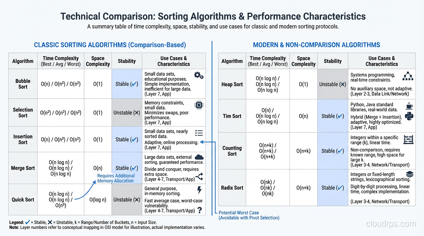
Best case: O(n) when the array is already sorted (with the early termination check). Worst case: O(n^2) for a reverse-sorted array. Space: O(1), sorts in place.

Bubble sort has one redeeming quality: it’s stable (equal elements maintain their relative order). Otherwise, it has no practical use. If you find bubble sort in production code, replace it immediately.

Insertion Sort: O(n^2), But Useful

Insertion sort builds the sorted array one element at a time, inserting each element into its correct position among the already-sorted elements.

def insertion_sort(arr):
    for i in range(1, len(arr)):
        key = arr[i]
        j = i - 1
        while j >= 0 and arr[j] > key:
            arr[j + 1] = arr[j]
            j -= 1
        arr[j + 1] = key
    return arr

Best case: O(n) when the array is already sorted. Worst case: O(n^2) for a reverse-sorted array. Space: O(1).

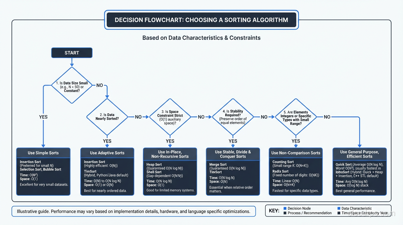
Despite its O(n^2) worst case, insertion sort has practical value. For small arrays (under 20-50 elements), the overhead of more complex algorithms exceeds the benefit of their better asymptotic complexity. This is why Timsort and introsort use insertion sort as a subroutine for small subsequences.

Insertion sort is also adaptive; its performance improves when the input is nearly sorted. For nearly sorted data, it approaches O(n), which makes it excellent for incremental sorting (adding a few elements to an already-sorted list).

Selection Sort: O(n^2), Rarely Useful

Selection sort finds the minimum element in the unsorted portion and places it at the beginning. It’s simple but performs O(n^2) comparisons regardless of input order, with no best-case improvement for sorted input.

The only niche use: when write operations are extremely expensive (like writing to flash memory with limited write cycles), selection sort minimizes swaps (exactly n-1 swaps, compared to O(n^2) for bubble sort).

The Efficient Sorts: What You Actually Use

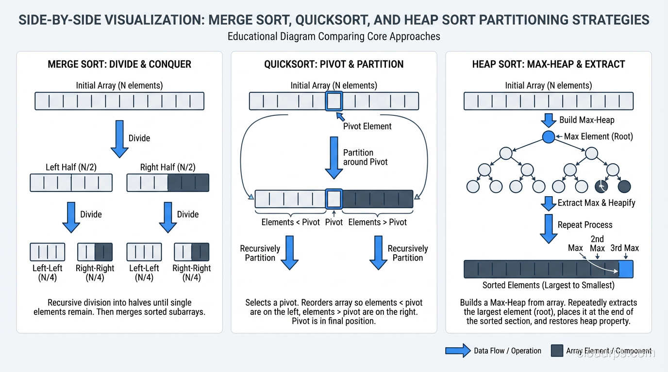
Merge Sort: O(n log n), Guaranteed

Merge sort divides the array in half, recursively sorts each half, then merges the sorted halves. It’s the quintessential divide-and-conquer algorithm.

def merge_sort(arr):
    if len(arr) <= 1:
        return arr
    mid = len(arr) // 2
    left = merge_sort(arr[:mid])
    right = merge_sort(arr[mid:])
    return merge(left, right)

def merge(left, right):
    result = []
    i = j = 0
    while i < len(left) and j < len(right):
        if left[i] <= right[j]:
            result.append(left[i])
            i += 1
        else:
            result.append(right[j])
            j += 1
    result.extend(left[i:])
    result.extend(right[j:])
    return result

Time: O(n log n) in all cases (best, worst, and average). Space: O(n), requires additional space for the merged output. Stable: Yes.

Merge sort’s guaranteed O(n log n) makes it the safe choice when predictable performance matters. It’s the default sort for linked lists (where random access is expensive, making quicksort less efficient). It’s also the basis for external sorting (sorting data that doesn’t fit in memory) because the merge operation works well with sequential I/O.

Quicksort: O(n log n) Average, O(n^2) Worst

Quicksort selects a “pivot” element, partitions the array into elements less than and greater than the pivot, then recursively sorts each partition.

def quicksort(arr):
    if len(arr) <= 1:
        return arr
    pivot = arr[len(arr) // 2]
    left = [x for x in arr if x < pivot]
    middle = [x for x in arr if x == pivot]
    right = [x for x in arr if x > pivot]
    return quicksort(left) + middle + quicksort(right)

Best/Average case: O(n log n). Worst case: O(n^2) when the pivot consistently selects the smallest or largest element (already-sorted input with naive pivot selection). Space: O(log n) for the recursion stack (in-place variant). Stable: No (in its standard form).

Despite the worse worst case compared to merge sort, quicksort is often faster in practice because of better cache behavior. Quicksort accesses memory sequentially within partitions, while merge sort’s merge phase accesses two separate arrays. On modern hardware with CPU caches, this locality difference can be 2-3x.

The worst-case problem is solved with randomized pivot selection or the median-of-three heuristic (pick the median of the first, middle, and last elements). With these improvements, the probability of hitting worst-case behavior is astronomically low.

Heap Sort: O(n log n), In-Place

Heap sort builds a max-heap from the array, then repeatedly extracts the maximum element. It’s O(n log n) worst case with O(1) extra space, which sounds like the perfect algorithm, but poor cache locality makes it slower than quicksort in practice.

Heap sort’s niche: when you need guaranteed O(n log n) with O(1) extra space. This combination is unique among comparison sorts.

The Production Sort: Timsort

Timsort, developed by Tim Peters for Python in 2002, is the sort behind Python’s sorted(), Java’s Arrays.sort() for objects, and many other standard libraries. It’s a hybrid of merge sort and insertion sort, designed for real-world data rather than theoretical inputs.

Key insights behind Timsort:

1. Real data has “runs”, sequences of already-sorted elements. Timsort identifies natural runs and merges them, rather than blindly dividing the array in half like merge sort.

2. Small subarrays are faster with insertion sort. Timsort uses insertion sort for runs shorter than a minimum length (typically 32-64 elements).

3. Merge strategy matters. Timsort maintains a stack of runs and merges them in a specific order that minimizes total comparisons while maintaining stability.

Time: O(n) best case (already sorted), O(n log n) worst case. Space: O(n). Stable: Yes.

The best-case O(n) for sorted input is a practical advantage that pure merge sort or quicksort don’t offer. Real datasets are often partially sorted (time-series data, log files, incrementally updated lists) and Timsort handles these efficiently.

Introsort: The Other Production Sort

C++ std::sort uses introsort, a hybrid of quicksort, heap sort, and insertion sort. It starts with quicksort, monitors the recursion depth, and switches to heap sort if the depth exceeds 2 * log(n) (preventing worst-case O(n^2) behavior). Small subarrays use insertion sort.

Introsort is not stable (it uses quicksort), but it doesn’t require extra memory (unlike Timsort’s O(n) space). The choice between Timsort and introsort in standard libraries reflects different priorities: stability and real-world performance (Timsort) vs minimal memory usage (introsort).

Non-Comparison Sorts: Breaking the O(n log n) Barrier

Counting Sort: O(n + k)

When your values are integers in a known, small range [0, k], counting sort counts occurrences of each value and reconstructs the sorted array. No comparisons needed.

Time: O(n + k) where k is the range of values. Space: O(k).

If k is comparable to n, this is effectively O(n), faster than any comparison sort. If k is much larger than n (sorting 100 integers in the range [0, 10 billion]), the space and time overhead makes it impractical.

Radix Sort: O(d * n)

Radix sort processes integers digit by digit, using a stable sort (usually counting sort) for each digit position. It’s O(d * n) where d is the number of digits.

For fixed-width integers (32-bit, 64-bit), d is constant, making radix sort effectively O(n). This is provably faster than comparison sorts and practical for sorting large arrays of integers.

I’ve used radix sort in performance-critical data pipelines processing millions of integer keys. The speedup over standard library sort was 3-4x for 64-bit integer arrays.

When Algorithm Choice Actually Matters

It Matters When:

• Dataset is large (millions of elements or more). The difference between O(n log n) and O(n^2) is the difference between seconds and days.
• Sort is called frequently (inner loop of a data pipeline, real-time system). Even a 2x improvement in sort performance matters when it runs thousands of times per second.
• Memory is constrained (embedded systems, very large datasets). Choosing between O(n) extra space (Timsort) and O(1) (heap sort) might be the deciding factor.
• Data has special properties (integers in a known range, nearly sorted). Specialized algorithms (radix sort, insertion sort) can dramatically outperform general-purpose sorts.

It Doesn’t Matter When:

• Dataset is small (under 10,000 elements). Every algorithm is fast enough. Use the standard library.
• Sort is called rarely (once at startup, once per user request). Even an inefficient sort is negligible in the overall request latency.
• The bottleneck is elsewhere (database queries, network I/O, serialization). Optimizing the sort won’t help if the program spends 95% of its time waiting on the network.

For scripting vs compiled language considerations: the standard library sort in Python (Timsort, implemented in C) is dramatically faster than any sort you implement in pure Python. Always prefer the built-in sort unless you have a very specific reason not to.

Sorting in Databases and Distributed Systems

Sorting at the application level is one thing. Sorting in databases and distributed systems introduces entirely different challenges.

Database sorting (ORDER BY) uses the query optimizer to choose between index scans (pre-sorted data, O(n)), in-memory sorts (quick for small result sets), and external sorts (merge sort variant for results that don’t fit in memory). Understanding this helps you write queries that sort efficiently. Sorting by an indexed column is dramatically faster than sorting by a computed expression.

Distributed sorting (MapReduce shuffle, Spark sort) partitions data across nodes, sorts locally on each node, then merges the sorted partitions. The network transfer during the shuffle phase dominates the cost. This is why partition design matters so much in big data. A bad partition key leads to data skew, which means one node sorts most of the data while others sit idle.

The Practical Takeaway

Use your language’s built-in sort. It’s been optimized by people who think about sorting algorithms for a living. It handles edge cases (empty arrays, single elements, already-sorted data) correctly. It’s stable (in Python and Java, at least).

Learn the algorithms not because you’ll implement them, but because understanding them gives you intuition about performance. When you see an ORDER BY on an unindexed column in a database query, you’ll know it’s triggering an O(n log n) sort. When you see nested loops comparing every element to every other element, you’ll recognize O(n^2) behavior. When someone suggests “just sort the data first,” you’ll know whether that’s a trivial operation or a significant computation.

That intuition, knowing when algorithm choice matters and when it doesn’t, is what separates experienced engineers from the rest.